Learning Algorithms
*“A computer program is said to learn from experience E with respect to some class of tasks T and performance measure P, if its performance at tasks in T, as measured by P, improves with experience E.” - Mitchell(1997)
The Task, *T
The task defines how the ML system should process a collection of features, an example.
Possible types of tasks are listed below.
Classification
The program has to assign an input to a category.
EX) Object recognition with image input
Sometimes, not every measurement of the input vector is provided. The program has to learn a set of functions, each function corresponding to classifying x with a different subset of its inputs missing.
Regression
The program has to predict a numerical value given some input.
EX) Future prices of securities
Transcription
The program has to observe a relatively unstructured representation of some kind of data and transcribe the information into discrete textual form.
EX) Speech recognition of an audio recording
Machine Translation
The program has to convert a sequence of symbols in some language into that in another language.
EX) Korean -> English
Structured Output
This kind of tasks involve any task where the output is a vector (or other data structure containing multiple values) with important relationships between the different elements. Transcription and translation tasks are also structured output tasks.
Anomaly Detection
The program has to shift through a set of events/objects and flag them if they are unusual/atypical.
Synthesis and Sampling
The program has to generate new examples that are similar to the given examples. There is no single correct output for each input.
EX) The program emits an audio waveform containing a spoken version of the given sentence.
Imputation of Missing Values
The program has to predict the values of the missing entries in a given example.
Density Estimation / Probability Mass Function Estimation
Denoising
The program has to predict the clean version of the corrupted example.
The Performance Measure, *P
Performance is a quantitative measure of how well the model carries out the task.
The accuracy, the proportion of examples for which the model produces the correct output, of the model is often measured for classification type of tasks. We can use the error rate or the 0-1 loss for equivalent information.
For tasks such as density estimation, the most common approach is to report the average log-probability the model assigns to some examples.
In many cases, it is complicated but is important to design a good aproximation to the deired criterion for measuring performance.
The Experience, *E
Most machine learning algorithms simply experience a dataset.
A dataset can be described with a design matrix, which is a matrix containing a different example in each row. Each column of a design matrix corresponds to a different feature.
Machine learning algorithms can be broadly categorized as unsupervised or supervised by what kind of experience they are allowed to have during the learning process.
Unsupervised Learning
Algorithms experience a dataset containing a large number of features, and then learn useful properties of the structure of the dataset.
Density estimation in support of other tasks is usually considered unsupervised learning.
Supervised Learning
Algorithms experience a dataset with a label/target associated with each example, and then learn to predict an output from an input. The design matrix also includes label/target in supervised learning.
Traditionally, regression, classification, and structured output tasks are considered supervised learning problems.
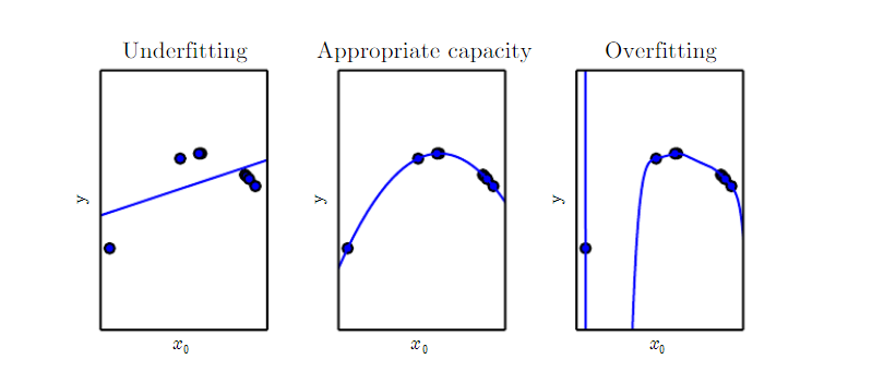
Capacity, Overfitting, and Underfitting
Generalization is the ability to perform well on new inputs.
In machine learning, we want to minimize the generalization error(test error) as well as the training error. We typically estimate the generalization error of a machine learning model by measuring its performance on a test set of examples that were collected separately from the training set.
Making the i.i.d. assumptions(1) the examples in the each dataset are independent from each other 2) the training set and test set are identically distributed), it is possible to describe the data-generating process with a probability distribution over a single example, calling it the data-generating distribution. By doing so, mathematically study the relationship between training error andtest error.
Thus, we can improve performance of the ML algorithm by
1) making the training error small
2) making the gap between the training and test error small
If the training error is not sufficiently low, the model is underfitted.
On the other hand, if the training error is low enough but the gap between the training error and the test error is too large, the model is overfitted.
We can control whether a model is more likely to overfit or underfit by altering its capacity, an ability to fit a wide variety of functions.
One way to control the capacity of a learning algorithm is by choosing its hypothesis space, the set of functions that the learning algorithm is allowed to select as being the solution.
EX) generalizing linear regression to include polynomials by changing the number of input features and adding parameters
The capacity of the model can be quantified with Vapnik-Chervonenkis dimension. The VC dimension measures the capacity of a binary classifier. The VC dimension is the largest possible number of the training set m, each of it having different x examples that the classifier can label arbitrarily.
By quantifying the capacity, we can see that the discrepancy between training error and generalization(test) error is bounded from above, and the bound goes up as the model capacity grows, but comes down as the number of training examples increases.
Expected generalization error can never increase as the number of training examples increases. For nonparametric (learning model with no previously fixed parameters) models, more data yield better generalization until the best possible error is achieved. Any fixed parametric model with less than optimal capacity will asymptote to an error value that exceeds the Bayes error(The error incurred by an oracle making predictions from the true distribution p(x, y)).
As the training size increases to infinity, the training error of any fixed-capacity model must rise to at least the Bayes error. As the training set size increases, the optimal capacity increases. The optimal capacity plateaus after reaching sufficient complexity to solve the task.
We can also control the capacity of the model through regularization. Regularization is any modification of model intended to reduce its generalization error but not its training error. This can be done by expressing a preference for one function to another, by adding a penalty called a regularizer.
Hyperparameters and Validation Sets
Hyperparameters are the settings we use to control the algorithm's behavior. If learned on the training set, such hyperparameters would always choose the maximum possible model capacity, resulting in overfitting.
For example, we can always fit the training set better with a higher-degree polynomial and a weight decay setting of λ= 0 than we could with a lower-degree polynomial and a positive weight decay setting.
To solve this problem, we need a validation set of examples that the training algorithm does not observe. The validation set is constructed from the training data(usually in 8:2 ratio of the total training set), because test exampes should not be used in any way to make choices about the model, including its hyperparameters. After all hyperparameter optimization is complete, the generalization error may be estimated using the test set.
Dividing the dataset into a fixed training set and a fixed test set can be problematic if it results in the test set being small. In this case, in order to estimate the test error more accurately, we can do cross-validation, repeating the training and testing computation on different randomly chosen subsets or splitsof the original dataset.
Estimators, Bias, and Variance
Estimators
Parameters are measured quantity of a population(a.k.a real world) that summarizes an aspect of the population. Population mean, standard deviation, a set of weights in the linear regression function can be the example of parameters.
Statistics/point estimators are used to estimate these population parameters. An estimator is a rule, a function for calculating an estimate from observed data, sample.
In other words, a point estimator is any function of m independent i.i.d data points:
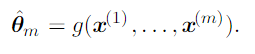
To distinguish estimates of parameters from their true value, we put a hat above.
According to this definition, any function could be an estimator. A good estimator is a function whose output, an estimate, is close to the true underlying θ, the population parameter.
Bias
Bias of an estimator is simply a difference between expected value of an estimate and parameter.
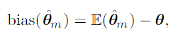
If bias of an estimator equals zero, an estimator is said to be unbiased.
In addition it is said to be asymptotically unbiased if bias of an estimator approaches to zero as a number of examples reaches infinity.
Variance and Standard Error
The variance, or the standard error, of an estimator provides a measure of how we would expect the estimate we compute from data to vary as we independently resample the dataset from the underlying data-generating process. Just as we might like an estimator to exhibit low bias, we would also like it to have relatively low variance.
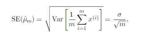
For most estimators, the variance of the estimator decreases as the number of examples in the dataset increases.
Trade-off of Bias and Variance
Bias measures the expected deviation from the true value of the parameter. Variance on the other hand, provides a measure of the deviation from the expected estimator value that any particular sampling of the data is likely to cause.
If we have to choose between an estimator with low bias but high variance and an estimator with low variance but high bias, we use cross-validation and compare the mean squared error(MSE).
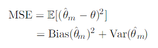
The MSE measures the overall expected deviation between the estimator and the true value of the parameter θ.
Consistency
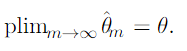
Consistency means convergence to the true value of the parameters as the number of data points in dataset increases to infinity.
The symbol plim indicates convergence in probability, meaning that as the number of data points in dataset increases to infinity, the probability that the difference between an estimate and true parameter is bigger than the noise converges to 0.
Consistency ensures that the bias induced by the estimator diminishes as the number of data examples grows, but reverse does not work.
The reason is that the convergence of expected value of the estimate to the real parameter does not guarantee the convergence of the estimate to the real parameter.
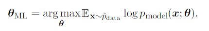
Maximum Likelihood Estimation
Maximum likelihood principle is a good criterion to choose which estimator we should consider.
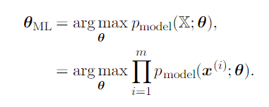
where X is a set of m examples drawn independently from the true but unknown data-generating distribution pdata(x), and pmodel(x;θ) is a parametric family of probability distributions over the same space indexed by θ.
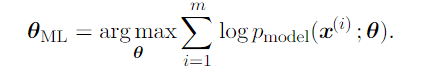
Then, we take log to transform product in to a sum.
Finally, we rescale the cost function to obtain a version of the criterion that is expressed as an expectation with respect to the empirical distribution defined by the training data.
One way to interpret maximum likelihood estimation is to view it as minimizingthe dissimilarity between the empirical distribution and the model distribution, with the degree of dissimilarity between the two measured by the KL divergence. The KL divergence is given by

and since what we are concerned with is the model, we only need to minimize
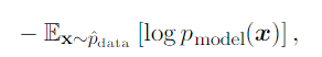
and doing so maximizeds the likelihood.
Minimizing this KL divergence corresponds exactly to minimizing the cross-entropy between the distributions.
Any loss consisting of a negative log-likelihood is a cross-entropy between the empirical distribution defined by the training set and the probability distribution defined by model.
p.130