# 데이터 전처리 패키지
import numpy as np #수치해석 패키지로 행렬식 계산할 때 주로 사용됨.
import pandas as pd #데이터를 엑셀과 같은 형태로 보여지도록 만들어주는 패키지

# 회귀모델 구축 및 평가 패키지
import statsmodels.formula.api as smf

# 데이터 시각화 패키지
import matplotlib.pyplot as plt
데이터 불러오기
-
1학기 동안 상받은 횟수와 성적 및 코스웍과의 관계
-
x변수가 총 2개 (독립변수)
- prog (코스웍)
- math (기말고사 수학성적)
-
y변수는 총 1개 (종속변수)
- num_awards (1학기 동안 상받은 횟수)
푸아송 및 음이항 회귀분석을 하기 위한 확인사항
1. 종속변수가 count variable 인가
2. 평균과 분산의 관계가 어떠한가 (같은지 분산이 더 큰지)
df = pd.read_csv('https://stats.idre.ucla.edu/stat/data/poisson_sim.csv')
df.head()| id | num_awards | prog | math | |
|---|---|---|---|---|
| 0 | 45 | 0 | 3 | 41 |
| 1 | 108 | 0 | 1 | 41 |
| 2 | 15 | 0 | 3 | 44 |
| 3 | 67 | 0 | 3 | 42 |
| 4 | 153 | 0 | 3 | 40 |
<svg xmlns="http://www.w3.org/2000/svg" height="24px"viewBox="0 0 24 24"
width="24px">
df.rename({'num awards':'num_awards'}, axis = 1, inplace = True)
df| id | num_awards | prog | math | |
|---|---|---|---|---|
| 0 | 45 | 0 | 3 | 41 |
| 1 | 108 | 0 | 1 | 41 |
| 2 | 15 | 0 | 3 | 44 |
| 3 | 67 | 0 | 3 | 42 |
| 4 | 153 | 0 | 3 | 40 |
| ... | ... | ... | ... | ... |
| 195 | 100 | 2 | 2 | 71 |
| 196 | 143 | 2 | 3 | 75 |
| 197 | 68 | 1 | 2 | 71 |
| 198 | 57 | 0 | 2 | 72 |
| 199 | 132 | 3 | 2 | 73 |
200 rows × 4 columns
<svg xmlns="http://www.w3.org/2000/svg" height="24px"viewBox="0 0 24 24"
width="24px">
df.columns = [col.replace(' ', '_') for col in df.columns]
df.columns
Index(['id', 'num_awards', 'prog', 'math'], dtype='object')df.describe() #각 변수별 수치해석을 보여줌 (샘플의 수, 평균, 표준편차, 최소 최댓값, 4분위수값)| id | num_awards | prog | math | |
|---|---|---|---|---|
| count | 200.000000 | 200.000000 | 200.000000 | 200.000000 |
| mean | 100.500000 | 0.630000 | 2.025000 | 52.645000 |
| std | 57.879185 | 1.052921 | 0.690477 | 9.368448 |
| min | 1.000000 | 0.000000 | 1.000000 | 33.000000 |
| 25% | 50.750000 | 0.000000 | 2.000000 | 45.000000 |
| 50% | 100.500000 | 0.000000 | 2.000000 | 52.000000 |
| 75% | 150.250000 | 1.000000 | 2.250000 | 59.000000 |
| max | 200.000000 | 6.000000 | 3.000000 | 75.000000 |
<svg xmlns="http://www.w3.org/2000/svg" height="24px"viewBox="0 0 24 24"
width="24px">
df.info() # 각 컬럼별로 결측치가 있는지, 데이터 타입은 무엇인지 등<class 'pandas.core.frame.DataFrame'>
RangeIndex: 200 entries, 0 to 199
Data columns (total 4 columns):
# Column Non-Null Count Dtype
--- ------ -------------- -----
0 id 200 non-null int64
1 num_awards 200 non-null int64
2 prog 200 non-null int64
3 math 200 non-null int64
dtypes: int64(4)
memory usage: 6.4 KB1. 종속변수가 count variable 인가
df['num_awards'].unique()array([0, 1, 3, 2, 5, 4, 6])2. 종속변수의 평균과 분산은?
model_nb = smf.negativebinomial('num_awards ~ math', data = df).fit() #음이항 회귀모델을 돌려보자
print(model_nb.summary())
Optimization terminated successfully.
Current function value: 0.940841
Iterations: 20
Function evaluations: 26
Gradient evaluations: 26
NegativeBinomial Regression Results
==============================================================================
Dep. Variable: num_awards No. Observations: 200
Model: NegativeBinomial Df Residuals: 198
Method: MLE Df Model: 1
Date: Mon, 12 Jun 2023 Pseudo R-squ.: 0.1343
Time: 04:07:07 Log-Likelihood: -188.17
converged: True LL-Null: -217.37
Covariance Type: nonrobust LLR p-value: 2.132e-14
==============================================================================
coef std err z P>|z| [0.025 0.975]
------------------------------------------------------------------------------
Intercept -5.4458 0.671 -8.121 0.000 -6.760 -4.132
math 0.0881 0.011 7.850 0.000 0.066 0.110
alpha 0.2694 0.177 1.518 0.129 -0.078 0.617
==============================================================================X와 y의 관계에 대해서 대략적으로 그림으로 살펴보기
- 수학성적과 상받은 횟수에 대한 관계(독립변수 1개만 고려)plt.figure(figsize = (5, 3))
plt.plot(df['math'], df['num_awards'], '*', alpha = 0.3)
plt.title('Math score and Number of received Awards')
plt.xlabel('Math Score')
plt.ylabel('Awards')
plt.show()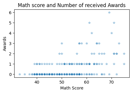
푸아송 회귀모델
model_poisson = smf.poisson('num_awards ~ math', data = df).fit()
print(model_poisson.summary())
Optimization terminated successfully.
Current function value: 0.950190
Iterations 6
Poisson Regression Results
==============================================================================
Dep. Variable: num_awards No. Observations: 200
Model: Poisson Df Residuals: 198
Method: MLE Df Model: 1
Date: Mon, 12 Jun 2023 Pseudo R-squ.: 0.1804
Time: 04:07:15 Log-Likelihood: -190.04
converged: True LL-Null: -231.86
Covariance Type: nonrobust LLR p-value: 5.903e-20
==============================================================================
coef std err z P>|z| [0.025 0.975]
------------------------------------------------------------------------------
Intercept -5.3335 0.591 -9.021 0.000 -6.492 -4.175
math 0.0862 0.010 8.902 0.000 0.067 0.105
==============================================================================푸아송 회귀모델
푸아송 확률함수
where ()
Incidence rate ratio (IRR)
- 독립변수가 1단위 증가할 때 단위시간당 평균발생횟수의 비율이 어떻게 변하는가?
IRR = np.exp(0.0862)
IRR #독립변수가 1단위 증가할 때 단위시간당 평균발생횟수가 어떻게 변하는가?1.0900243113683694수학성적이 1점 증가할때 1학기 평균 상받는 횟수는 1.09배 만큼 증가한다.
실제 데이터와 구한 푸아송 회귀모델 그림그리기
X = df['math'].sort_values()
y = np.exp(-5.3335 + 0.0862 * X) #푸아송 회귀모델plt.figure(figsize = (5, 3))
plt.plot(df['math'], df['num_awards'], 'go', alpha = 0.3, label = 'True data')
plt.plot(X, y, linewidth = 3, label = 'Poisson Regression Line')
plt.title('Math score and Number of received Awards')
plt.xlabel('Math Score')
plt.ylabel('Awards')
plt.legend()
plt.tight_layout()
plt.show()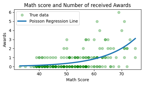
포아송회귀모델과 음이항회귀모델의 비교
model_nb.params #음이항 모델의 회귀계수 뽑기Intercept -5.445762
math 0.088123
alpha 0.269401
dtype: float64- 푸아송모델:
- 음이항모델:

Deep Learning, Multi-Agent RL, Large Language Model, Statistics