Logistic Regression

Jihwan Oh·2023년 12월 13일

Logistic Regression iris dataset sigmoid function statsmodels

data analysis

목록 보기

6/9

# 데이터 전처리 패키지
import numpy as np #수치해석 패키지로 행렬식 계산할 때 주로 사용됨.
import pandas as pd #데이터를 엑셀과 같은 형태로 보여지도록 만들어주는 패키지

# 회귀모델 구축 및 평가 패키지
import statsmodels #다양한 통계검정과 추정에 필요한 기능을 제공
import statsmodels.formula.api as smf

# 데이터 시각화 패키지
import matplotlib.pyplot as plt

데이터 불러오기

붓꽃데이터
x변수가 총 4개 (독립변수)
- sepal length
- sepal width
- petal length
- width width
y변수는 총 3개 (독립변수)
- 'setosa'
- 'versicolor'
- 'virginica'

from sklearn.datasets import load_iris #sklearn 데이터셋에서 제공해주는 붓꽃데이터 사용
iris = load_iris()
print(iris)

{'data': array([[5.1, 3.5, 1.4, 0.2],
       [4.9, 3. , 1.4, 0.2],
       [4.7, 3.2, 1.3, 0.2],
       [4.6, 3.1, 1.5, 0.2],
       [5. , 3.6, 1.4, 0.2],
       [5.4, 3.9, 1.7, 0.4],
       [4.6, 3.4, 1.4, 0.3],
       [5. , 3.4, 1.5, 0.2],
       [4.4, 2.9, 1.4, 0.2],
       [4.9, 3.1, 1.5, 0.1],
       [5.4, 3.7, 1.5, 0.2],
       [4.8, 3.4, 1.6, 0.2],
       [4.8, 3. , 1.4, 0.1],
       [4.3, 3. , 1.1, 0.1],
       [5.8, 4. , 1.2, 0.2],
       [5.7, 4.4, 1.5, 0.4],
       [5.4, 3.9, 1.3, 0.4],
       [5.1, 3.5, 1.4, 0.3],
       [5.7, 3.8, 1.7, 0.3],
       [5.1, 3.8, 1.5, 0.3],
       [5.4, 3.4, 1.7, 0.2],
       [5.1, 3.7, 1.5, 0.4],
       [4.6, 3.6, 1. , 0.2],
       [5.1, 3.3, 1.7, 0.5],
       [4.8, 3.4, 1.9, 0.2],
       [5. , 3. , 1.6, 0.2],
       [5. , 3.4, 1.6, 0.4],
       [5.2, 3.5, 1.5, 0.2],
       [5.2, 3.4, 1.4, 0.2],
       [4.7, 3.2, 1.6, 0.2],
       [4.8, 3.1, 1.6, 0.2],
       [5.4, 3.4, 1.5, 0.4],
       [5.2, 4.1, 1.5, 0.1],
       [5.5, 4.2, 1.4, 0.2],
       [4.9, 3.1, 1.5, 0.2],
       [5. , 3.2, 1.2, 0.2],
       [5.5, 3.5, 1.3, 0.2],
       [4.9, 3.6, 1.4, 0.1],
       [4.4, 3. , 1.3, 0.2],
       [5.1, 3.4, 1.5, 0.2],
       [5. , 3.5, 1.3, 0.3],
       [4.5, 2.3, 1.3, 0.3],
       [4.4, 3.2, 1.3, 0.2],
       [5. , 3.5, 1.6, 0.6],
       [5.1, 3.8, 1.9, 0.4],
       [4.8, 3. , 1.4, 0.3],
       [5.1, 3.8, 1.6, 0.2],
       [4.6, 3.2, 1.4, 0.2],
       [5.3, 3.7, 1.5, 0.2],
       [5. , 3.3, 1.4, 0.2],
       [7. , 3.2, 4.7, 1.4],
       [6.4, 3.2, 4.5, 1.5],
       [6.9, 3.1, 4.9, 1.5],
       [5.5, 2.3, 4. , 1.3],
       [6.5, 2.8, 4.6, 1.5],
       [5.7, 2.8, 4.5, 1.3],
       [6.3, 3.3, 4.7, 1.6],
       [4.9, 2.4, 3.3, 1. ],
       [6.6, 2.9, 4.6, 1.3],
       [5.2, 2.7, 3.9, 1.4],
       [5. , 2. , 3.5, 1. ],
       [5.9, 3. , 4.2, 1.5],
       [6. , 2.2, 4. , 1. ],
       [6.1, 2.9, 4.7, 1.4],
       [5.6, 2.9, 3.6, 1.3],
       [6.7, 3.1, 4.4, 1.4],
       [5.6, 3. , 4.5, 1.5],
       [5.8, 2.7, 4.1, 1. ],
       [6.2, 2.2, 4.5, 1.5],
       [5.6, 2.5, 3.9, 1.1],
       [5.9, 3.2, 4.8, 1.8],
       [6.1, 2.8, 4. , 1.3],
       [6.3, 2.5, 4.9, 1.5],
       [6.1, 2.8, 4.7, 1.2],
       [6.4, 2.9, 4.3, 1.3],
       [6.6, 3. , 4.4, 1.4],
       [6.8, 2.8, 4.8, 1.4],
       [6.7, 3. , 5. , 1.7],
       [6. , 2.9, 4.5, 1.5],
       [5.7, 2.6, 3.5, 1. ],
       [5.5, 2.4, 3.8, 1.1],
       [5.5, 2.4, 3.7, 1. ],
       [5.8, 2.7, 3.9, 1.2],
       [6. , 2.7, 5.1, 1.6],
       [5.4, 3. , 4.5, 1.5],
       [6. , 3.4, 4.5, 1.6],
       [6.7, 3.1, 4.7, 1.5],
       [6.3, 2.3, 4.4, 1.3],
       [5.6, 3. , 4.1, 1.3],
       [5.5, 2.5, 4. , 1.3],
       [5.5, 2.6, 4.4, 1.2],
       [6.1, 3. , 4.6, 1.4],
       [5.8, 2.6, 4. , 1.2],
       [5. , 2.3, 3.3, 1. ],
       [5.6, 2.7, 4.2, 1.3],
       [5.7, 3. , 4.2, 1.2],
       [5.7, 2.9, 4.2, 1.3],
       [6.2, 2.9, 4.3, 1.3],
       [5.1, 2.5, 3. , 1.1],
       [5.7, 2.8, 4.1, 1.3],
       [6.3, 3.3, 6. , 2.5],
       [5.8, 2.7, 5.1, 1.9],
       [7.1, 3. , 5.9, 2.1],
       [6.3, 2.9, 5.6, 1.8],
       [6.5, 3. , 5.8, 2.2],
       [7.6, 3. , 6.6, 2.1],
       [4.9, 2.5, 4.5, 1.7],
       [7.3, 2.9, 6.3, 1.8],
       [6.7, 2.5, 5.8, 1.8],
       [7.2, 3.6, 6.1, 2.5],
       [6.5, 3.2, 5.1, 2. ],
       [6.4, 2.7, 5.3, 1.9],
       [6.8, 3. , 5.5, 2.1],
       [5.7, 2.5, 5. , 2. ],
       [5.8, 2.8, 5.1, 2.4],
       [6.4, 3.2, 5.3, 2.3],
       [6.5, 3. , 5.5, 1.8],
       [7.7, 3.8, 6.7, 2.2],
       [7.7, 2.6, 6.9, 2.3],
       [6. , 2.2, 5. , 1.5],
       [6.9, 3.2, 5.7, 2.3],
       [5.6, 2.8, 4.9, 2. ],
       [7.7, 2.8, 6.7, 2. ],
       [6.3, 2.7, 4.9, 1.8],
       [6.7, 3.3, 5.7, 2.1],
       [7.2, 3.2, 6. , 1.8],
       [6.2, 2.8, 4.8, 1.8],
       [6.1, 3. , 4.9, 1.8],
       [6.4, 2.8, 5.6, 2.1],
       [7.2, 3. , 5.8, 1.6],
       [7.4, 2.8, 6.1, 1.9],
       [7.9, 3.8, 6.4, 2. ],
       [6.4, 2.8, 5.6, 2.2],
       [6.3, 2.8, 5.1, 1.5],
       [6.1, 2.6, 5.6, 1.4],
       [7.7, 3. , 6.1, 2.3],
       [6.3, 3.4, 5.6, 2.4],
       [6.4, 3.1, 5.5, 1.8],
       [6. , 3. , 4.8, 1.8],
       [6.9, 3.1, 5.4, 2.1],
       [6.7, 3.1, 5.6, 2.4],
       [6.9, 3.1, 5.1, 2.3],
       [5.8, 2.7, 5.1, 1.9],
       [6.8, 3.2, 5.9, 2.3],
       [6.7, 3.3, 5.7, 2.5],
       [6.7, 3. , 5.2, 2.3],
       [6.3, 2.5, 5. , 1.9],
       [6.5, 3. , 5.2, 2. ],
       [6.2, 3.4, 5.4, 2.3],
       [5.9, 3. , 5.1, 1.8]]), 'target': array([0, 0, 0, 0, 0, 0, 0, 0, 0, 0, 0, 0, 0, 0, 0, 0, 0, 0, 0, 0, 0, 0,
       0, 0, 0, 0, 0, 0, 0, 0, 0, 0, 0, 0, 0, 0, 0, 0, 0, 0, 0, 0, 0, 0,
       0, 0, 0, 0, 0, 0, 1, 1, 1, 1, 1, 1, 1, 1, 1, 1, 1, 1, 1, 1, 1, 1,
       1, 1, 1, 1, 1, 1, 1, 1, 1, 1, 1, 1, 1, 1, 1, 1, 1, 1, 1, 1, 1, 1,
       1, 1, 1, 1, 1, 1, 1, 1, 1, 1, 1, 1, 2, 2, 2, 2, 2, 2, 2, 2, 2, 2,
       2, 2, 2, 2, 2, 2, 2, 2, 2, 2, 2, 2, 2, 2, 2, 2, 2, 2, 2, 2, 2, 2,
       2, 2, 2, 2, 2, 2, 2, 2, 2, 2, 2, 2, 2, 2, 2, 2, 2, 2]), 'frame': None, 'target_names': array(['setosa', 'versicolor', 'virginica'], dtype='<U10'), 'DESCR': '.. _iris_dataset:\n\nIris plants dataset\n--------------------\n\n**Data Set Characteristics:**\n\n    :Number of Instances: 150 (50 in each of three classes)\n    :Number of Attributes: 4 numeric, predictive attributes and the class\n    :Attribute Information:\n        - sepal length in cm\n        - sepal width in cm\n        - petal length in cm\n        - petal width in cm\n        - class:\n                - Iris-Setosa\n                - Iris-Versicolour\n                - Iris-Virginica\n                \n    :Summary Statistics:\n\n    ============== ==== ==== ======= ===== ====================\n                    Min  Max   Mean    SD   Class Correlation\n    ============== ==== ==== ======= ===== ====================\n    sepal length:   4.3  7.9   5.84   0.83    0.7826\n    sepal width:    2.0  4.4   3.05   0.43   -0.4194\n    petal length:   1.0  6.9   3.76   1.76    0.9490  (high!)\n    petal width:    0.1  2.5   1.20   0.76    0.9565  (high!)\n    ============== ==== ==== ======= ===== ====================\n\n    :Missing Attribute Values: None\n    :Class Distribution: 33.3% for each of 3 classes.\n    :Creator: R.A. Fisher\n    :Donor: Michael Marshall (MARSHALL%PLU@io.arc.nasa.gov)\n    :Date: July, 1988\n\nThe famous Iris database, first used by Sir R.A. Fisher. The dataset is taken\nfrom Fisher\'s paper. Note that it\'s the same as in R, but not as in the UCI\nMachine Learning Repository, which has two wrong data points.\n\nThis is perhaps the best known database to be found in the\npattern recognition literature.  Fisher\'s paper is a classic in the field and\nis referenced frequently to this day.  (See Duda & Hart, for example.)  The\ndata set contains 3 classes of 50 instances each, where each class refers to a\ntype of iris plant.  One class is linearly separable from the other 2; the\nlatter are NOT linearly separable from each other.\n\n.. topic:: References\n\n   - Fisher, R.A. "The use of multiple measurements in taxonomic problems"\n     Annual Eugenics, 7, Part II, 179-188 (1936); also in "Contributions to\n     Mathematical Statistics" (John Wiley, NY, 1950).\n   - Duda, R.O., & Hart, P.E. (1973) Pattern Classification and Scene Analysis.\n     (Q327.D83) John Wiley & Sons.  ISBN 0-471-22361-1.  See page 218.\n   - Dasarathy, B.V. (1980) "Nosing Around the Neighborhood: A New System\n     Structure and Classification Rule for Recognition in Partially Exposed\n     Environments".  IEEE Transactions on Pattern Analysis and Machine\n     Intelligence, Vol. PAMI-2, No. 1, 67-71.\n   - Gates, G.W. (1972) "The Reduced Nearest Neighbor Rule".  IEEE Transactions\n     on Information Theory, May 1972, 431-433.\n   - See also: 1988 MLC Proceedings, 54-64.  Cheeseman et al"s AUTOCLASS II\n     conceptual clustering system finds 3 classes in the data.\n   - Many, many more ...', 'feature_names': ['sepal length (cm)', 'sepal width (cm)', 'petal length (cm)', 'petal width (cm)'], 'filename': 'iris.csv', 'data_module': 'sklearn.datasets.data'}

데이터 전처리

iris.feature_names #독립변수명

['sepal length (cm)',
 'sepal width (cm)',
 'petal length (cm)',
 'petal width (cm)']

독립변수, 종속변수 분리

X = iris.data #독립변수
y = iris.target #종속변수
print(X)
# print(y)

[[5.1 3.5 1.4 0.2]
 [4.9 3.  1.4 0.2]
 [4.7 3.2 1.3 0.2]
 [4.6 3.1 1.5 0.2]
 [5.  3.6 1.4 0.2]
 [5.4 3.9 1.7 0.4]
 [4.6 3.4 1.4 0.3]
 [5.  3.4 1.5 0.2]
 [4.4 2.9 1.4 0.2]
 [4.9 3.1 1.5 0.1]
 [5.4 3.7 1.5 0.2]
 [4.8 3.4 1.6 0.2]
 [4.8 3.  1.4 0.1]
 [4.3 3.  1.1 0.1]
 [5.8 4.  1.2 0.2]
 [5.7 4.4 1.5 0.4]
 [5.4 3.9 1.3 0.4]
 [5.1 3.5 1.4 0.3]
 [5.7 3.8 1.7 0.3]
 [5.1 3.8 1.5 0.3]
 [5.4 3.4 1.7 0.2]
 [5.1 3.7 1.5 0.4]
 [4.6 3.6 1.  0.2]
 [5.1 3.3 1.7 0.5]
 [4.8 3.4 1.9 0.2]
 [5.  3.  1.6 0.2]
 [5.  3.4 1.6 0.4]
 [5.2 3.5 1.5 0.2]
 [5.2 3.4 1.4 0.2]
 [4.7 3.2 1.6 0.2]
 [4.8 3.1 1.6 0.2]
 [5.4 3.4 1.5 0.4]
 [5.2 4.1 1.5 0.1]
 [5.5 4.2 1.4 0.2]
 [4.9 3.1 1.5 0.2]
 [5.  3.2 1.2 0.2]
 [5.5 3.5 1.3 0.2]
 [4.9 3.6 1.4 0.1]
 [4.4 3.  1.3 0.2]
 [5.1 3.4 1.5 0.2]
 [5.  3.5 1.3 0.3]
 [4.5 2.3 1.3 0.3]
 [4.4 3.2 1.3 0.2]
 [5.  3.5 1.6 0.6]
 [5.1 3.8 1.9 0.4]
 [4.8 3.  1.4 0.3]
 [5.1 3.8 1.6 0.2]
 [4.6 3.2 1.4 0.2]
 [5.3 3.7 1.5 0.2]
 [5.  3.3 1.4 0.2]
 [7.  3.2 4.7 1.4]
 [6.4 3.2 4.5 1.5]
 [6.9 3.1 4.9 1.5]
 [5.5 2.3 4.  1.3]
 [6.5 2.8 4.6 1.5]
 [5.7 2.8 4.5 1.3]
 [6.3 3.3 4.7 1.6]
 [4.9 2.4 3.3 1. ]
 [6.6 2.9 4.6 1.3]
 [5.2 2.7 3.9 1.4]
 [5.  2.  3.5 1. ]
 [5.9 3.  4.2 1.5]
 [6.  2.2 4.  1. ]
 [6.1 2.9 4.7 1.4]
 [5.6 2.9 3.6 1.3]
 [6.7 3.1 4.4 1.4]
 [5.6 3.  4.5 1.5]
 [5.8 2.7 4.1 1. ]
 [6.2 2.2 4.5 1.5]
 [5.6 2.5 3.9 1.1]
 [5.9 3.2 4.8 1.8]
 [6.1 2.8 4.  1.3]
 [6.3 2.5 4.9 1.5]
 [6.1 2.8 4.7 1.2]
 [6.4 2.9 4.3 1.3]
 [6.6 3.  4.4 1.4]
 [6.8 2.8 4.8 1.4]
 [6.7 3.  5.  1.7]
 [6.  2.9 4.5 1.5]
 [5.7 2.6 3.5 1. ]
 [5.5 2.4 3.8 1.1]
 [5.5 2.4 3.7 1. ]
 [5.8 2.7 3.9 1.2]
 [6.  2.7 5.1 1.6]
 [5.4 3.  4.5 1.5]
 [6.  3.4 4.5 1.6]
 [6.7 3.1 4.7 1.5]
 [6.3 2.3 4.4 1.3]
 [5.6 3.  4.1 1.3]
 [5.5 2.5 4.  1.3]
 [5.5 2.6 4.4 1.2]
 [6.1 3.  4.6 1.4]
 [5.8 2.6 4.  1.2]
 [5.  2.3 3.3 1. ]
 [5.6 2.7 4.2 1.3]
 [5.7 3.  4.2 1.2]
 [5.7 2.9 4.2 1.3]
 [6.2 2.9 4.3 1.3]
 [5.1 2.5 3.  1.1]
 [5.7 2.8 4.1 1.3]
 [6.3 3.3 6.  2.5]
 [5.8 2.7 5.1 1.9]
 [7.1 3.  5.9 2.1]
 [6.3 2.9 5.6 1.8]
 [6.5 3.  5.8 2.2]
 [7.6 3.  6.6 2.1]
 [4.9 2.5 4.5 1.7]
 [7.3 2.9 6.3 1.8]
 [6.7 2.5 5.8 1.8]
 [7.2 3.6 6.1 2.5]
 [6.5 3.2 5.1 2. ]
 [6.4 2.7 5.3 1.9]
 [6.8 3.  5.5 2.1]
 [5.7 2.5 5.  2. ]
 [5.8 2.8 5.1 2.4]
 [6.4 3.2 5.3 2.3]
 [6.5 3.  5.5 1.8]
 [7.7 3.8 6.7 2.2]
 [7.7 2.6 6.9 2.3]
 [6.  2.2 5.  1.5]
 [6.9 3.2 5.7 2.3]
 [5.6 2.8 4.9 2. ]
 [7.7 2.8 6.7 2. ]
 [6.3 2.7 4.9 1.8]
 [6.7 3.3 5.7 2.1]
 [7.2 3.2 6.  1.8]
 [6.2 2.8 4.8 1.8]
 [6.1 3.  4.9 1.8]
 [6.4 2.8 5.6 2.1]
 [7.2 3.  5.8 1.6]
 [7.4 2.8 6.1 1.9]
 [7.9 3.8 6.4 2. ]
 [6.4 2.8 5.6 2.2]
 [6.3 2.8 5.1 1.5]
 [6.1 2.6 5.6 1.4]
 [7.7 3.  6.1 2.3]
 [6.3 3.4 5.6 2.4]
 [6.4 3.1 5.5 1.8]
 [6.  3.  4.8 1.8]
 [6.9 3.1 5.4 2.1]
 [6.7 3.1 5.6 2.4]
 [6.9 3.1 5.1 2.3]
 [5.8 2.7 5.1 1.9]
 [6.8 3.2 5.9 2.3]
 [6.7 3.3 5.7 2.5]
 [6.7 3.  5.2 2.3]
 [6.3 2.5 5.  1.9]
 [6.5 3.  5.2 2. ]
 [6.2 3.4 5.4 2.3]
 [5.9 3.  5.1 1.8]]

dfX = pd.DataFrame(X, columns=iris.feature_names) #데이터 프레임화
dfy = pd.DataFrame(y, columns=["species"])

단순로지스틱 회귀모델

df = pd.concat([dfX, dfy], axis=1) #독립변수 데이터,종속변수 데이터 하나로 합치기속변수 데이터 하나로 합치기, axis 는 열방향(0)으로 또는 행방향(1)으로 합칠지
df = df[["sepal length (cm)", "species"]] #독립변수는 'sepal length' 하나만
df

	sepal length (cm)	species
0	5.1	0
1	4.9	0
2	4.7	0
3	4.6	0
4	5.0	0
...	...	...
145	6.7	2
146	6.3	2
147	6.5	2
148	6.2	2
149	5.9	2

150 rows × 2 columns

df = df[df.species.isin([0, 1])] # 종속변수는 0, 1에 해당하는 것만 사용(이진변수로 만들기 위해) 0= setosa, 1 = versicolor
df = df.rename(columns={"sepal length (cm)": "sepal_length" }) #컬럼 이름 바꿔주기
df

	sepal_length	species
0	5.1	0
1	4.9	0
2	4.7	0
3	4.6	0
4	5.0	0
...	...	...
95	5.7	1
96	5.7	1
97	6.2	1
98	5.1	1
99	5.7	1

100 rows × 2 columns

model = smf.logit("species ~ sepal_length", data=df).fit() #로지스틱 모델 최적화

Optimization terminated successfully.
         Current function value: 0.321056
         Iterations 8

print(model.summary()) #결과정리

                           Logit Regression Results                           
==============================================================================
Dep. Variable:                species   No. Observations:                  100
Model:                          Logit   Df Residuals:                       98
Method:                           MLE   Df Model:                            1
Date:                Thu, 25 May 2023   Pseudo R-squ.:                  0.5368
Time:                        05:09:56   Log-Likelihood:                -32.106
converged:                       True   LL-Null:                       -69.315
Covariance Type:            nonrobust   LLR p-value:                 6.320e-18
================================================================================
                   coef    std err          z      P>|z|      [0.025      0.975]
--------------------------------------------------------------------------------
Intercept      -27.8315      5.434     -5.122      0.000     -38.481     -17.182
sepal_length     5.1403      1.007      5.107      0.000       3.168       7.113
================================================================================

Logit $\equiv$ $\beta_{0} + \beta_{1}x_{i}=-27.8315+5.1403x_{i}$

Logistic function $f(x_{i})=\frac{1}{1+e^{27.8315-5.1403x}}$

model.params #모델 파라미터

Intercept      -27.831451
sepal_length     5.140336
dtype: float64

Odds Ratio = $e^{\beta_{n}}$

odds_ratio = np.exp(model.params) #승산비율
print(odds_ratio)

Intercept       8.183789e-13
sepal_length    1.707732e+02
dtype: float64

데이터 시각화하기

sorted_x = df['sepal_length'].sort_values() #데이터 시각화를 위한 x값 오름차순 정렬
y = 1/(1+np.exp(27.831451 - 5.140336 * sorted_x)) # 데이터 x를 우리가 구한 로지스틱함수를 통해 y 값구하기

plt.figure(figsize=(10, 4)) #그림의 전체 크기 조정 (가로, 세로)

plt.plot(df['sepal_length'], df['species'], 'o', alpha = 0.5, label = 'true data') #실제 데이터
plt.plot(sorted_x, y, label = 'logistic function', linewidth = 3) #우리가 추측한 로지스틱 함수
plt.axhline(0.5, color='lightgray', linestyle='--', linewidth=2, label = 'threshold(0.5)')
plt.title('Logistic Regression')
plt.legend()
plt.xlabel('sepal_length')
plt.ylabel('setosa(0) or versicolor(1)')
plt.tight_layout()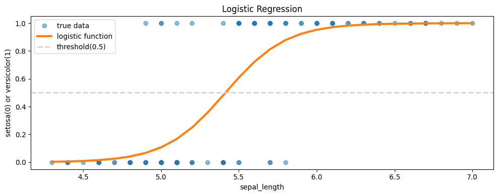

다중로지스틱 회귀모델

df = pd.concat([dfX, dfy], axis=1) #독립변수 데이터,종속변수 데이터 하나로 합치기속변수 데이터 하나로 합치기, axis 는 열방향으로 또는 행방향으로 합칠지
df

	sepal length (cm)	sepal width (cm)	petal length (cm)	petal width (cm)	species
0	5.1	3.5	1.4	0.2	0
1	4.9	3.0	1.4	0.2	0
2	4.7	3.2	1.3	0.2	0
3	4.6	3.1	1.5	0.2	0
4	5.0	3.6	1.4	0.2	0
...	...	...	...	...	...
145	6.7	3.0	5.2	2.3	2
146	6.3	2.5	5.0	1.9	2
147	6.5	3.0	5.2	2.0	2
148	6.2	3.4	5.4	2.3	2
149	5.9	3.0	5.1	1.8	2

150 rows × 5 columns

df.columns #데이터 프레임 컬럼명 확인

Index(['sepal length (cm)', 'sepal width (cm)', 'petal length (cm)',
       'petal width (cm)', 'species'],
      dtype='object')

df = df.rename(columns = {df.columns[0]: 'sepal_length',  #데이터 컬럼명 바꿔주기
                     df.columns[1]: 'sepal_width',
                     df.columns[2]: 'petal_length',
                     df.columns[3]: 'petal_width'})
df

	sepal_length	sepal_width	petal_length	petal_width	species
0	5.1	3.5	1.4	0.2	0
1	4.9	3.0	1.4	0.2	0
2	4.7	3.2	1.3	0.2	0
3	4.6	3.1	1.5	0.2	0
4	5.0	3.6	1.4	0.2	0
...	...	...	...	...	...
145	6.7	3.0	5.2	2.3	2
146	6.3	2.5	5.0	1.9	2
147	6.5	3.0	5.2	2.0	2
148	6.2	3.4	5.4	2.3	2
149	5.9	3.0	5.1	1.8	2

150 rows × 5 columns

df = df[df.species.isin([1, 2])] # 종속변수는 1, 2에 해당하는 것만 사용(이진변수로 만들기 위해)  1 = versicolor, 2 = virginicaf
df['species'] -= 1 #df['scpecies'] = df['species'] - 1 #statsmodels에서 로지스틱 회귀를 할 때는 종속변수 값이 반드시 0과 1로만 구성되어 있어야해서 1을 빼주는 작업
df
# df = pd.concat([df.drop(['species'], axis = 1), df.species-1], axis = 1) # 1을 빼는 또다른 방법

df['species'] -= 1 #df['scpecies'] = df['species'] - 1 #statsmodels에서 로지스틱 회귀를 할 때는 종속변수 값이 반드시 0과 1로만 구성되어 있어야해서 1을 빼주는 작업

	sepal_length	sepal_width	petal_length	petal_width	species
50	7.0	3.2	4.7	1.4	0
51	6.4	3.2	4.5	1.5	0
52	6.9	3.1	4.9	1.5	0
53	5.5	2.3	4.0	1.3	0
54	6.5	2.8	4.6	1.5	0
...	...	...	...	...	...
145	6.7	3.0	5.2	2.3	1
146	6.3	2.5	5.0	1.9	1
147	6.5	3.0	5.2	2.0	1
148	6.2	3.4	5.4	2.3	1
149	5.9	3.0	5.1	1.8	1

100 rows × 5 columns

model = smf.logit("species ~ sepal_length + sepal_width + petal_length + petal_width", data = df).fit() #모델 만들기
print(model.summary())

Optimization terminated successfully.
         Current function value: 0.059493
         Iterations 12
                           Logit Regression Results                           
==============================================================================
Dep. Variable:                species   No. Observations:                  100
Model:                          Logit   Df Residuals:                       95
Method:                           MLE   Df Model:                            4
Date:                Thu, 25 May 2023   Pseudo R-squ.:                  0.9142
Time:                        05:09:57   Log-Likelihood:                -5.9493
converged:                       True   LL-Null:                       -69.315
Covariance Type:            nonrobust   LLR p-value:                 1.947e-26
================================================================================
                   coef    std err          z      P>|z|      [0.025      0.975]
--------------------------------------------------------------------------------
Intercept      -42.6378     25.708     -1.659      0.097     -93.024       7.748
sepal_length    -2.4652      2.394     -1.030      0.303      -7.158       2.228
sepal_width     -6.6809      4.480     -1.491      0.136     -15.461       2.099
petal_length     9.4294      4.737      1.990      0.047       0.145      18.714
petal_width     18.2861      9.743      1.877      0.061      -0.809      37.381
================================================================================

Possibly complete quasi-separation: A fraction 0.60 of observations can be
perfectly predicted. This might indicate that there is complete
quasi-separation. In this case some parameters will not be identified.

Logit $\equiv$ $\beta_{0} + \beta_{1}x_{1} + \beta_{2}x_{2} + \beta_{3}x_{3} + \beta_{4}x_{4}=-42.6378-2.4652x_{1}-6.6809x_{2}+9.4294x_{3}+18.2861x_{4}$

Logistic function $f(x_{i})=\frac{1}{1+e^{42.6378+2.4652x_{1}+6.6809x_{2}-9.4294x_{3}-18.2861x_{4}}}$

Odds Ratio = $e^{\beta_{n}}$

odds_ratio = np.exp(model.params) #승산비율
print(odds_ratio)

Intercept       3.038345e-19
sepal_length    8.499013e-02
sepal_width     1.254665e-03
petal_length    1.244887e+04
petal_width     8.741145e+07
dtype: float64

Jihwan Oh

Deep Learning, Multi-Agent RL, Large Language Model, Statistics

이전 포스트

Regression (회귀분석)

다음 포스트

Logistic Regression

data analysis

데이터 불러오기

데이터 전처리

독립변수, 종속변수 분리

단순로지스틱 회귀모델

Logit $\equiv$ $\beta_{0} + \beta_{1}x_{i}=-27.8315+5.1403x_{i}$

Logistic function $f(x_{i})=\frac{1}{1+e^{27.8315-5.1403x}}$

Odds Ratio = $e^{\beta_{n}}$

데이터 시각화하기

다중로지스틱 회귀모델

Logit $\equiv$ $\beta_{0} + \beta_{1}x_{1} + \beta_{2}x_{2} + \beta_{3}x_{3} + \beta_{4}x_{4}=-42.6378-2.4652x_{1}-6.6809x_{2}+9.4294x_{3}+18.2861x_{4}$

Logistic function $f(x_{i})=\frac{1}{1+e^{42.6378+2.4652x_{1}+6.6809x_{2}-9.4294x_{3}-18.2861x_{4}}}$

Odds Ratio = $e^{\beta_{n}}$

Regression (회귀분석)

Count Variable(Poisson or Negative Binomial regression)

0개의 댓글

관련 채용 정보

	sepal length (cm)	species
0	5.1	0
1	4.9	0
2	4.7	0
3	4.6	0
4	5.0	0
...	...	...
145	6.7	2
146	6.3	2
147	6.5	2
148	6.2	2
149	5.9	2

	sepal_length	species
0	5.1	0
1	4.9	0
2	4.7	0
3	4.6	0
4	5.0	0
...	...	...
95	5.7	1
96	5.7	1
97	6.2	1
98	5.1	1
99	5.7	1

	sepal length (cm)	sepal width (cm)	petal length (cm)	petal width (cm)	species
0	5.1	3.5	1.4	0.2	0
1	4.9	3.0	1.4	0.2	0
2	4.7	3.2	1.3	0.2	0
3	4.6	3.1	1.5	0.2	0
4	5.0	3.6	1.4	0.2	0
...	...	...	...	...	...
145	6.7	3.0	5.2	2.3	2
146	6.3	2.5	5.0	1.9	2
147	6.5	3.0	5.2	2.0	2
148	6.2	3.4	5.4	2.3	2
149	5.9	3.0	5.1	1.8	2

	sepal_length	sepal_width	petal_length	petal_width	species
0	5.1	3.5	1.4	0.2	0
1	4.9	3.0	1.4	0.2	0
2	4.7	3.2	1.3	0.2	0
3	4.6	3.1	1.5	0.2	0
4	5.0	3.6	1.4	0.2	0
...	...	...	...	...	...
145	6.7	3.0	5.2	2.3	2
146	6.3	2.5	5.0	1.9	2
147	6.5	3.0	5.2	2.0	2
148	6.2	3.4	5.4	2.3	2
149	5.9	3.0	5.1	1.8	2

	sepal_length	sepal_width	petal_length	petal_width	species
50	7.0	3.2	4.7	1.4	0
51	6.4	3.2	4.5	1.5	0
52	6.9	3.1	4.9	1.5	0
53	5.5	2.3	4.0	1.3	0
54	6.5	2.8	4.6	1.5	0
...	...	...	...	...	...
145	6.7	3.0	5.2	2.3	1
146	6.3	2.5	5.0	1.9	1
147	6.5	3.0	5.2	2.0	1
148	6.2	3.4	5.4	2.3	1
149	5.9	3.0	5.1	1.8	1

	sepal length (cm)	species
0	5.1	0
1	4.9	0
2	4.7	0
3	4.6	0
4	5.0	0
...	...	...
145	6.7	2
146	6.3	2
147	6.5	2
148	6.2	2
149	5.9	2

	sepal_length	species
0	5.1	0
1	4.9	0
2	4.7	0
3	4.6	0
4	5.0	0
...	...	...
95	5.7	1
96	5.7	1
97	6.2	1
98	5.1	1
99	5.7	1

	sepal length (cm)	sepal width (cm)	petal length (cm)	petal width (cm)	species
0	5.1	3.5	1.4	0.2	0
1	4.9	3.0	1.4	0.2	0
2	4.7	3.2	1.3	0.2	0
3	4.6	3.1	1.5	0.2	0
4	5.0	3.6	1.4	0.2	0
...	...	...	...	...	...
145	6.7	3.0	5.2	2.3	2
146	6.3	2.5	5.0	1.9	2
147	6.5	3.0	5.2	2.0	2
148	6.2	3.4	5.4	2.3	2
149	5.9	3.0	5.1	1.8	2

	sepal_length	sepal_width	petal_length	petal_width	species
0	5.1	3.5	1.4	0.2	0
1	4.9	3.0	1.4	0.2	0
2	4.7	3.2	1.3	0.2	0
3	4.6	3.1	1.5	0.2	0
4	5.0	3.6	1.4	0.2	0
...	...	...	...	...	...
145	6.7	3.0	5.2	2.3	2
146	6.3	2.5	5.0	1.9	2
147	6.5	3.0	5.2	2.0	2
148	6.2	3.4	5.4	2.3	2
149	5.9	3.0	5.1	1.8	2

	sepal_length	sepal_width	petal_length	petal_width	species
50	7.0	3.2	4.7	1.4	0
51	6.4	3.2	4.5	1.5	0
52	6.9	3.1	4.9	1.5	0
53	5.5	2.3	4.0	1.3	0
54	6.5	2.8	4.6	1.5	0
...	...	...	...	...	...
145	6.7	3.0	5.2	2.3	1
146	6.3	2.5	5.0	1.9	1
147	6.5	3.0	5.2	2.0	1
148	6.2	3.4	5.4	2.3	1
149	5.9	3.0	5.1	1.8	1

Logistic Regression

data analysis

데이터 불러오기

데이터 전처리

독립변수, 종속변수 분리

단순로지스틱 회귀모델

Logit ≡\equiv≡ β0+β1xi=−27.8315+5.1403xi\beta_{0} + \beta_{1}x_{i}=-27.8315+5.1403x_{i}β0​+β1​xi​=−27.8315+5.1403xi​

Logistic function f(xi)=11+e27.8315−5.1403xf(x_{i})=\frac{1}{1+e^{27.8315-5.1403x}}f(xi​)=1+e27.8315−5.1403x1​

Odds Ratio = eβne^{\beta_{n}}eβn​

데이터 시각화하기

다중로지스틱 회귀모델

Logistic function f(xi)=11+e42.6378+2.4652x1+6.6809x2−9.4294x3−18.2861x4f(x_{i})=\frac{1}{1+e^{42.6378+2.4652x_{1}+6.6809x_{2}-9.4294x_{3}-18.2861x_{4}}}f(xi​)=1+e42.6378+2.4652x1​+6.6809x2​−9.4294x3​−18.2861x4​1​

Odds Ratio = eβne^{\beta_{n}}eβn​

Regression (회귀분석)

Count Variable(Poisson or Negative Binomial regression)

0개의 댓글

관련 채용 정보

Logit $\equiv$ $\beta_{0} + \beta_{1}x_{i}=-27.8315+5.1403x_{i}$

Logistic function $f(x_{i})=\frac{1}{1+e^{27.8315-5.1403x}}$

Odds Ratio = $e^{\beta_{n}}$

Logistic function $f(x_{i})=\frac{1}{1+e^{42.6378+2.4652x_{1}+6.6809x_{2}-9.4294x_{3}-18.2861x_{4}}}$

Odds Ratio = $e^{\beta_{n}}$

	sepal length (cm)	species
0	5.1	0
1	4.9	0
2	4.7	0
3	4.6	0
4	5.0	0
...	...	...
145	6.7	2
146	6.3	2
147	6.5	2
148	6.2	2
149	5.9	2

	sepal_length	species
0	5.1	0
1	4.9	0
2	4.7	0
3	4.6	0
4	5.0	0
...	...	...
95	5.7	1
96	5.7	1
97	6.2	1
98	5.1	1
99	5.7	1

	sepal length (cm)	sepal width (cm)	petal length (cm)	petal width (cm)	species
0	5.1	3.5	1.4	0.2	0
1	4.9	3.0	1.4	0.2	0
2	4.7	3.2	1.3	0.2	0
3	4.6	3.1	1.5	0.2	0
4	5.0	3.6	1.4	0.2	0
...	...	...	...	...	...
145	6.7	3.0	5.2	2.3	2
146	6.3	2.5	5.0	1.9	2
147	6.5	3.0	5.2	2.0	2
148	6.2	3.4	5.4	2.3	2
149	5.9	3.0	5.1	1.8	2

	sepal_length	sepal_width	petal_length	petal_width	species
0	5.1	3.5	1.4	0.2	0
1	4.9	3.0	1.4	0.2	0
2	4.7	3.2	1.3	0.2	0
3	4.6	3.1	1.5	0.2	0
4	5.0	3.6	1.4	0.2	0
...	...	...	...	...	...
145	6.7	3.0	5.2	2.3	2
146	6.3	2.5	5.0	1.9	2
147	6.5	3.0	5.2	2.0	2
148	6.2	3.4	5.4	2.3	2
149	5.9	3.0	5.1	1.8	2

	sepal_length	sepal_width	petal_length	petal_width	species
50	7.0	3.2	4.7	1.4	0
51	6.4	3.2	4.5	1.5	0
52	6.9	3.1	4.9	1.5	0
53	5.5	2.3	4.0	1.3	0
54	6.5	2.8	4.6	1.5	0
...	...	...	...	...	...
145	6.7	3.0	5.2	2.3	1
146	6.3	2.5	5.0	1.9	1
147	6.5	3.0	5.2	2.0	1
148	6.2	3.4	5.4	2.3	1
149	5.9	3.0	5.1	1.8	1