Diffusion Model
Diffusion 모델은 Forward Process로 매 timestep t마다 추가한 Gaussian noise q(xt∣xt−1)를 다시 pθ(xt−1∣xt)로 복원하는 과정인 Backward Process를 학습하는 생성모델 알고리즘이다.
1) Score-Based generative model: learn to model distributions with increasing levels of Gaussian noise

2) use annealed Langevin dynamics: undo this noise
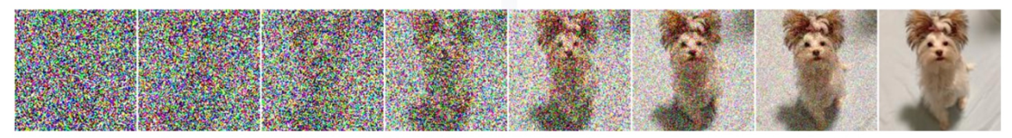
image gradually appears out of Gaussian noise
Diffusion 모델은 이 두 과정을 각각 forward/backward process의 개념으로 정의하고 사용한다.
1) gradually turning data to noise, and 2) learning the inverse of this process.

iterative하게 시행
Markov Chain
: Markov 성질을 갖는 이산확률과정
- Markov 성질: “특정 상태의 확률(t+1)은 오직 현재(t)의 상태에 의존한다”
- 이산확률과정: 이산적인 시간(0초, 1초, 2초, ..) 속에서의 확률적 현상
P[st+1∣st]=P[st+1∣s1,..,t]
ex. “내일의 날씨는 오늘의 날씨만 보고 알 수 있다.” (내일의 날씨는 오로지 오늘의 날씨 만을 조건부로 하는 확률적 과정)
Forward process q(xt∣xt−1)
- defined by user
- score-based model의 annealing과 유사
Steps
- data sample x0∼q(x0)
- Markov chain : gradually adds noise to the data, producing sequence of increasingly noisy samples x1,…xT
- at each step t, we sample xt from the following Markov operator
q(xt∣xt−1)=N(xt;αtxt−1,1−αtI)
where αt∈(0,1),αt→0
alpha는 noise 주입 정도이다.
- 최종 xT는 standard Gaussian distribution N(0,1).
q(x1:T∣x0):=t=1∏Tq(xt∣xt−1)q(xt∣xt−1):=N(xt;1−βtxt−1,βtI)
- Gaussian Distribution(N)에서 나온 noise를 data에 더해준다.
- q(x1:T∣x0) 수식을 보면, 우도(likelihood)의 형태를 보이고 있다.
- β는 diffusion rate(variance schedule)로 분산이 divergence하는 것을 방지해준다.
- 하지만 위의 β를 이용해서 수식을 전개하면 0~T의 모든 수식을 step by step으로 전개해야 하여 메모리 소모가 크고 시간도 오래 걸린다.
- 이를 해소하기 위해 α를 이용한다.
αt:=1−βt and αˉt:=s=1∏tαsq(xt∣x0)=N(xt;αˉtx0,(1−αˉt)I)
- xt는 Gaussian Distribution에서 나오는 값이기 때문에 평균을 기준으로 어느 정도 분산으로 치우친 값을 가질 것이다.
- α를 이용하여 한 번에 전개가 가능하다.
T steps of diffusion
q(x(0⋯T))=q(x(0))t=1∏Tq(x(t)∣x(t−1))
xt=αtxt−1+1−αtϵt=αtαt−1xt−2+1−αtαt−1ϵt=…=αˉtx0+1−αˉtϵt∼N(0,I)ϵ∼N(0,I)
첫 번째줄: definition of Markov operator (next xt = previous xt + gaussian noise with extra multiplier that is defined by the schedule)
x0을 얻을 때까지 반복한다.
최종 형태: rescaled x0 + gaussian noise (scheduling variables 포함)
q(xt∣x0)=N(xt;αˉtx0,(1−αˉt)I)
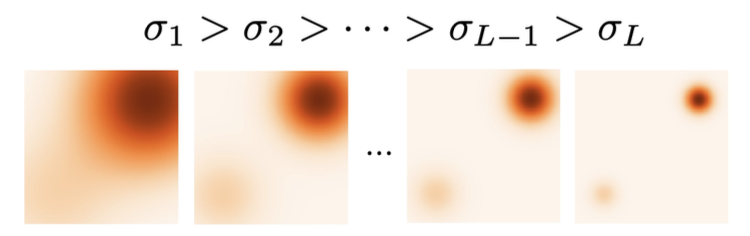
annealed langevin dynamics
기존 space에 noise를 점진적으로 추가하는 과정이다. #Forward Process
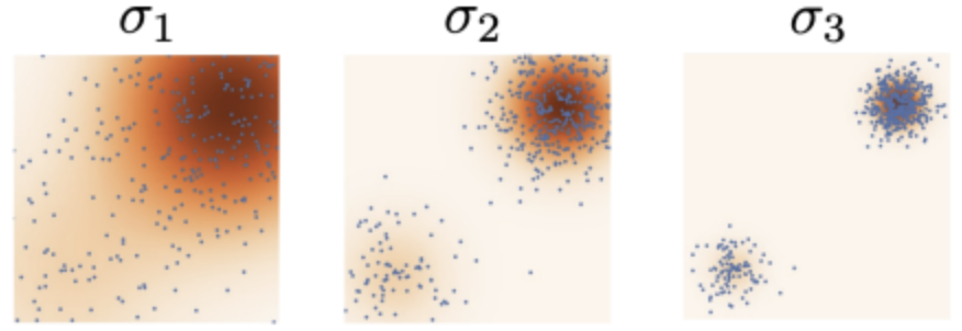
처음에는 큰 노이즈를 추가하고, 뒤로 갈수록 노이즈의 양을 줄여 모델이 데이터 군집을 제대로 향하도록 유도한다.
이 노이즈를 제거해 원하는 데이터를 추출할 수 있다. #Backward Process
Backward process p(xt−1∣xt) : Diffusion Process
get the inverse of the above Markov chain
Gaussian noise를 제거해가며 특정한 패턴을 만들어가는 과정이다.
우리는 이 process를 알지는 못하지만 데이터로부터 학습할 수 있도록 할 것이다.
Model:
backward process를 학습하는 Diffusion 모델의 확률 분포
pθ(x0:T)=p(xT)t=1∏Tpθ(xt−1∣xt)
pθ(xt−1∣xt)=N(xt−1;μθ(xt,t),Σθ(xt,t))
우리는 이미지 x0을 얻을 때까지 pθ(xt−1∣xt) 로부터 noise xT를 샘플링한다.
여기서 학습 대상은 μθ(xt,t),Σθ(xt,t) 이다.
평균과 분산을 잘 근사할 수 있도록 학습시킨다.
우리는 q(xt∣xt−1)으로부터 p(xt−1∣xt)를 학습시키는 것이 목표다.
따라서 pθ(xt−1∣xt)가 q(xt∣xt−1)에 근사해야 하고, 분포 차이를 최소화하는 KL Divergence로 학습 목표를 나타낼 수 있다.
DKL(q(x1:T∣x0)∥pθ(x1:T∣x0)
log likelihood
data point x0에서의 likelihood
evidence p(x0)의 lower bound
logpθ(x0)≥logpθ(x0)−DKL(q(x1:T∣x0)∥pθ(x1:T∣x0))=logpθ(x0)−Ex1:T∼q(x1:T∣x0)[logpθ(x0:T)/pθ(x0)q(x1:T∣x0)]=logpθ(x0)−Eq[logpθ(x0:T)q(x1:T∣x0)+logpθ(x0)]=−Eq[logpθ(x0:T)q(x1:T∣x0)]
Diffusion 모델의 ELBO
Eq[logpθ(x0:T)q(x1:T∣x0)]
이를 최대화하면,
p(x0)를 최대화하고 DKL(q(x1:T∣x0)∥pθ(x1:T∣x0)를 최소화시킬 수 있다.
VAE와 learning objective가 유사한데, pθ만을 최적화시킨다는 점이 다르다.
Loss Function : diffusion loss
위의 log likelihood를 최대화시키는 것이 목적
Eq[LTDKL(q(xT∣x0)∥pθ(xT))+t=2∑TLt−1DKL(q(xt−1∣xt,x0)∥pθ(xt−1∣xt))L0−logpθ(x0∣x1)]
- The prior loss (Regularization)
LT=DKL(q(xT∣x0)∥pθ(xT))
compares final xT and is often zero by construction
모델의 입력분포 p가 노이즈의 집합인 q를 잘 표현하는지를 측정, 알맞게 설정한 경우 0에 수렴한다.
- The reconstruction term
L0=−logpθ(x0∣x1)
is the probability of the true x0 given the model’s “best guess” x1.
모델의 최종 출력결과인 x1과 원본 데이터인 x0을 비교해 모델이 원본 데이터를 얼마나 잘 복원했는지 측정한다. 잘 학습되었을수록 0에 수렴한다.
- diffusion loss
Lt=DKL(q(xt∣xt+1,x0)∥pθ(xt∣xt+1)) for 1≤t≤T−1
measure whether the learned backward process pθ(xt∣xt+1) looks like the real backward process q(xt∣xt+1,x0).
학습된 backward process인 pθ(xt∣xt+1)가 실제 backward process인 q(xt∣xt+1,x0)를 얼마나 잘 근사하는지 측정한다.
Diffusion loss가 작을수록 noise가 잘 제거된다는 뜻이다.
Noise Parameterization : denoise from the noisy data
diffusion loss Lt을 noise parameterization을 수행함으로써 정규화시킬 수 있다. 최종적으로는 noisy data를 denoise시키는 작업으로 볼 수 있다.
앞서 Forward Process에서 q(xt∣x0)=N(xt;αˉtx0,(1−αˉt)I)를 증명했다.
정의와 베이즈정리를 통해, q(xt−1∣xt,x0)와 pθ(xt−1∣xt)가 모두 가우시안 분포를 따른다는 것을 알 수 있다. 따라서, 목적식을 가우시안 분포 간의 KL divergence로 다시 나타낼 수 있다.
μ~t=αt1(xt−1−αˉt1−αtϵt)
μθ(xt,t)=αt1(xt−1−αˉt1−αtϵθ(xt,t))
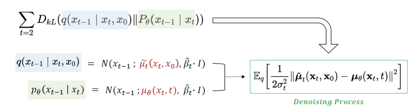
Lt=Ex0,ϵ[C1⋅∥μ~t(xt,x0)−μθ(xt,t)∥2]=Ex0,ϵ[C2⋅∥ϵt−ϵθ(xt,t)∥2]=Ex0,ϵ[C2⋅∥∥∥ϵt−ϵθ(αˉtx0+1−αˉtϵt,t)∥∥∥2]
(C1과 C2는 >0인 상수)
Diffusion training process
- Sample a datapoint x0
- Sample a time step t uniformly from 1,2,..., T.
- Sample noise ϵ∼N(0,I)
- Generate noisy xt=αˉtx0+1−αˉtϵt
- Take a gradient step on ∥ϵt−ϵθ(xt,t)∥2
- repeat until convergence
Ancestral Sampling : 새로운 데이터 생성
Diffusion process:
pθ(x0:T)=p(xT)t=1∏Tpθ(xt−1∣xt)
이 모델을 통해 데이터 xt−1을 생성할 수 있다.
xt−1∼pθ(xt−t∣xt) for t=T,T−1,…,1
sampling process for a diffusion model:
xt−1=αt1(xt−1−αˉt1−αtϵθ(xt,t))+σt⋅z
for t∈{T,T−1,…,1}
Ancestral Sampling vs. Langevin Dynamics
- recall that in Langevin Dynamics we repeatedly perform the update:
xt=xt−1+2αtsθ(x,σℓ)+αtϵt
- recall that score model sθ(x~) and the denoiser ϵ(x~) are related:
sθ(x~)≈∇x~logqσ(x~∣x)=σϵ≈1−αˉtϵ(x~)
xnew =x+2αt∇xlogpθ(x)+αtϵt
- recall sampling process for a diffusion model:
xt−1=αt1(xt−1−αˉt1−αtϵθ(xt,t))+σt⋅z
결국 annealed Langevin dynamics랑 형태가 같다.
Conditional diffusion model
y(label, noised image)가 주어지면 이미지 x를 생성하는 모델로 활용된다.
∇xlogp(x∣y)=∇xlogp(x)+∇xlogp(y∣x)
우변은 이미 알고 있는 정보 -> Langevin dynamics를 통해 좌변을 샘플링할 수 있다.
Variational Diffusion model, Latent Diffusion model로 응용될 수 있다.
참고: Cornell Tech CS 6785 Lecture 13
