Analysis of Variance and Design of Experiments
Design of Experiments
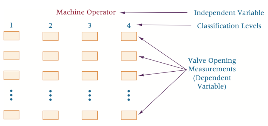
Experimental Design(실험계획): a plan and a structure to test hypotheses in which the experimenter either controls or manipulates one or more variables
ANOVA
Analysis of Variance (분산분석)dependent variable responses (measurements, data) are not all the same in a given study
ANOVA의 세 가지 종류
The Completely Randomized Design (CRD)
독립변수 하나
그 독립변수가 2 이상의 treatment level(or classification) 가짐
만약 treatment level이 2개라면, 이전처럼 t test 사용.
One-way ANOVA
: A hypothesis testing technique that is used to compare the
SSE(Error Sum of Squares) : The error variance, or that portion of the total variance unexplained by the treatmentSSC(Treatment Sum of Squares) : The variance resulting from the treatment(columns)SST(Total Sum of Squares): SST = SSC + SSE
∑ j = 1 C ∑ i = 1 n j ( x i j − x ˉ ) 2 = ∑ j = 1 C n j ( x ˉ j − x ˉ ) 2 + ∑ j = 1 C ∑ i = 1 n j ( x i j − x ˉ j ) 2 \sum_{j=1}^C \sum_{i=1}^{n_j}\left(x_{i j}-\bar{x}\right)^2=\sum_{j=1}^C n_j\left(\bar{x}_j-\bar{x}\right)^2+\sum_{j=1}^C \sum_{i=1}^{n_j}\left(x_{i j}-\bar{x}_j\right)^2 j = 1 ∑ C i = 1 ∑ n j ( x i j − x ˉ ) 2 = j = 1 ∑ C n j ( x ˉ j − x ˉ ) 2 + j = 1 ∑ C i = 1 ∑ n j ( x i j − x ˉ j ) 2 C C C j j j n j n_j n j i i i x ˉ \bar x x ˉ x ˉ j \bar x_j x ˉ j x i j x_{ij} x i j
the mean square of columns
M S C = S S C C − 1 \mathrm{MSC}=\frac{\mathrm{SSC}}{C-1} M S C = C − 1 S S C the mean square error
M S E = S S E N − C \mathrm{MSE}=\frac{\mathrm{SSE}}{N-C} M S E = N − C S S E ratio of the treatment variance to the error variance
F = M S C M S E \mathrm{F}=\frac{\mathrm{MSC}}{\mathrm{MSE}} F = M S E M S C df
( d f ) C = C − 1 ( d f ) E = N − C ( d f ) T = N − 1 \begin{aligned} & (\mathrm{df})_C=C-1 \\ & (\mathrm{df})_E=N-C \\ & (\mathrm{df})_T=N-1 \end{aligned} ( d f ) C = C − 1 ( d f ) E = N − C ( d f ) T = N − 1
Step 1.
H 0 : μ 1 = μ 2 = ⋯ = μ k H_0: \mu_1=\mu_2=\cdots=\mu_k H 0 : μ 1 = μ 2 = ⋯ = μ k H a : H_a: H a :
Step 2.
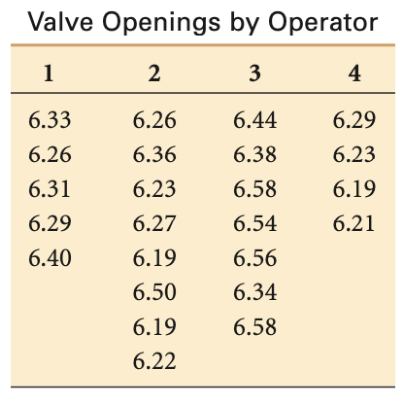
S S C = ∑ j = 1 C n j ( x ˉ j − x ˉ ) 2 \mathrm{SSC}=\sum_{j=1}^C n_j\left(\bar{x}_j-\bar{x}\right)^2 S S C = j = 1 ∑ C n j ( x ˉ j − x ˉ ) 2 S S E = ∑ i = 1 n j ∑ j = 1 C ( x i j − x ˉ j ) 2 \mathrm{SSE}=\sum_{i=1}^{n_j} \sum_{j=1}^C\left(x_{i j}-\bar{x}_j\right)^2 S S E = i = 1 ∑ n j j = 1 ∑ C ( x i j − x ˉ j ) 2 S S T = ∑ i = 1 n j ∑ j = 1 C ( x i j − x ˉ ) 2 \mathrm{SST}=\sum_{i=1}^{n_j} \sum_{j=1}^C\left(x_{i j}-\bar{x}\right)^2 S S T = i = 1 ∑ n j j = 1 ∑ C ( x i j − x ˉ ) 2 SSC = ∑ j = 1 C n j ( x ˉ j − x ˉ ) 2 = [ 5 ( 6.318 − 6.339583 ) 2 + 8 ( 6.2775 − 6.339583 ) 2 + 7 ( 6.488571 − 6.339583 ) 2 + 4 ( 6.230 − 6.339583 ) 2 ] = 0.00233 + 0.03083 + 0.15538 + 0.04803 = 0.23658 SSE = ∑ i = 1 n j ∑ j = 1 C ( x i j − x ˉ j ) 2 = [ ( 6.33 − 6.318 ) 2 + ( 6.26 − 6.318 ) 2 + ( 6.31 − 6.318 ) 2 + ( 6.29 − 6.318 ) 2 + ( 6.40 − 6.318 ) 2 + ( 6.26 − 6.2775 ) 2 + ( 6.36 − 6.2775 ) 2 + … + ( 6.19 − 6.230 ) 2 + ( 6.21 − 6.230 ) 2 = 0.15492 SST = ∑ i = 1 n j ∑ j = 1 C ( x i j − x ˉ ) 2 = [ ( 6.33 − 6.339583 ) 2 + ( 6.26 − 6.339583 ) 2 + ( 6.31 − 6.339583 ) 2 + … + ( 6.19 − 6.339583 ) 2 + ( 6.21 − 6.339583 ) 2 = 0.39150 \begin{aligned} \text { SSC }=\sum_{j=1}^C n_j\left(\bar{x}_j-\bar{x}\right)^2= & {\left[5(6.318-6.339583)^2+8(6.2775-6.339583)^2\right.} \\ & \left.+7(6.488571-6.339583)^2+4(6.230-6.339583)^2\right] \\ = & 0.00233+0.03083+0.15538+0.04803 \\ = & 0.23658 \\ \text { SSE }=\sum_{i=1}^{n_j} \sum_{j=1}^C\left(x_{i j}-\bar{x}_j\right)^2= & {\left[(6.33-6.318)^2+(6.26-6.318)^2+(6.31-6.318)^2\right.} \\ & +(6.29-6.318)^2+(6.40-6.318)^2+(6.26-6.2775)^2 \\ & +(6.36-6.2775)^2+\ldots+(6.19-6.230)^2+(6.21-6.230)^2 \\ = & 0.15492 \\ \text { SST }=\sum_{i=1}^{n_j} \sum_{j=1}^C\left(x_{i j}-\bar{x}\right)^2= & {\left[(6.33-6.339583)^2+(6.26-6.339583)^2\right.} \\ & +(6.31-6.339583)^2+\ldots+(6.19-6.339583)^2 \\ & +(6.21-6.339583)^2 \\ = & 0.39150 \end{aligned} SSC = j = 1 ∑ C n j ( x ˉ j − x ˉ ) 2 = = = SSE = i = 1 ∑ n j j = 1 ∑ C ( x i j − x ˉ j ) 2 = = SST = i = 1 ∑ n j j = 1 ∑ C ( x i j − x ˉ ) 2 = = [ 5 ( 6 . 3 1 8 − 6 . 3 3 9 5 8 3 ) 2 + 8 ( 6 . 2 7 7 5 − 6 . 3 3 9 5 8 3 ) 2 + 7 ( 6 . 4 8 8 5 7 1 − 6 . 3 3 9 5 8 3 ) 2 + 4 ( 6 . 2 3 0 − 6 . 3 3 9 5 8 3 ) 2 ] 0 . 0 0 2 3 3 + 0 . 0 3 0 8 3 + 0 . 1 5 5 3 8 + 0 . 0 4 8 0 3 0 . 2 3 6 5 8 [ ( 6 . 3 3 − 6 . 3 1 8 ) 2 + ( 6 . 2 6 − 6 . 3 1 8 ) 2 + ( 6 . 3 1 − 6 . 3 1 8 ) 2 + ( 6 . 2 9 − 6 . 3 1 8 ) 2 + ( 6 . 4 0 − 6 . 3 1 8 ) 2 + ( 6 . 2 6 − 6 . 2 7 7 5 ) 2 + ( 6 . 3 6 − 6 . 2 7 7 5 ) 2 + … + ( 6 . 1 9 − 6 . 2 3 0 ) 2 + ( 6 . 2 1 − 6 . 2 3 0 ) 2 0 . 1 5 4 9 2 [ ( 6 . 3 3 − 6 . 3 3 9 5 8 3 ) 2 + ( 6 . 2 6 − 6 . 3 3 9 5 8 3 ) 2 + ( 6 . 3 1 − 6 . 3 3 9 5 8 3 ) 2 + … + ( 6 . 1 9 − 6 . 3 3 9 5 8 3 ) 2 + ( 6 . 2 1 − 6 . 3 3 9 5 8 3 ) 2 0 . 3 9 1 5 0 Step 3.
d f C = C − 1 = 4 − 1 = 3 d f E = N − C = 24 − 4 = 20 d f T = N − 1 = 24 − 1 = 23 M S C = S S C d f C = . 23658 3 = . 078860 M S E = S S E d f E = . 15492 20 = . 007746 F = . 078860 . 007746 = 10.18 \begin{aligned} \mathrm{df}_C & =C-1=4-1=3 \\ \mathrm{df}_E & =N-C=24-4=20 \\ \mathrm{df}_T & =N-1=24-1=23 \\ \mathrm{MSC} & =\frac{\mathrm{SSC}}{\mathrm{df}_C}=\frac{.23658}{3}=.078860 \\ \mathrm{MSE} & =\frac{\mathrm{SSE}}{\mathrm{df}_E}=\frac{.15492}{20}=.007746 \\ F & =\frac{.078860}{.007746}=10.18 \end{aligned} d f C d f E d f T M S C M S E F = C − 1 = 4 − 1 = 3 = N − C = 2 4 − 4 = 2 0 = N − 1 = 2 4 − 1 = 2 3 = d f C S S C = 3 . 2 3 6 5 8 = . 0 7 8 8 6 0 = d f E S S E = 2 0 . 1 5 4 9 2 = . 0 0 7 7 4 6 = . 0 0 7 7 4 6 . 0 7 8 8 6 0 = 1 0 . 1 8 Step 4. ANOVA Table
Source of Variance df SS MS F Between 3 0.23658 0.078860 10.18 Error 20 0.15492 0.007746 Total 23 0.39150 \begin{array}{lrccc} \text { Source of Variance } & \text { df } & \text { SS } & \text { MS } & \text { F } \\ \hline \text { Between } & 3 & 0.23658 & 0.078860 & 10.18 \\ \text { Error } & 20 & 0.15492 & 0.007746 & \\ \text { Total } & 23 & 0.39150 & & \end{array} Source of Variance Between Error Total df 3 2 0 2 3 SS 0 . 2 3 6 5 8 0 . 1 5 4 9 2 0 . 3 9 1 5 0 MS 0 . 0 7 8 8 6 0 0 . 0 0 7 7 4 6 F 1 0 . 1 8 Step 5.
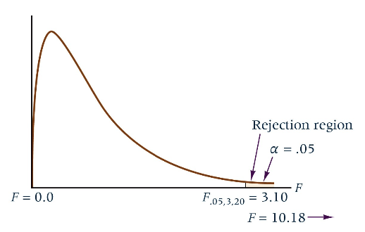
The observed F value of 10.187 is larger than the critical F value of 3.10(F 0.05 , 3 , 20 F_{0.05, 3, 20} F 0 . 0 5 , 3 , 2 0
H 0 H_0 H 0 The result indicates that not all means are equal, and there is a significant difference in the mean valve openings by machine operator
Multiple Comparison Tests
일원분산분석 결과 귀무가설이 기각되어 모집단의 평균 중에는 차이가 존재한다고 결론을 내리게 되면, 그 차이를 보이는 모집단이 어떤 것들인지에 대한 분석이 추가적으로 필요하다. 이를 다중비교라고 한다.
determine from the data which pairs of means are significantly different.
Tukey's Honestly Significant Difference (HSD) test
모든 가능한 조합의 평균 차이에 대한 신뢰구간을 고려한다. 만일 5개의 모집단을 다중비교하려면 5C2 = 10개 비교를 하면 된다.
Tukey’s HSD test requires equal sample sizes for all treatments
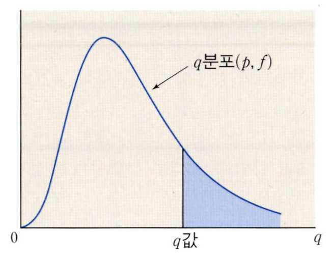
Tukey’s HSD test uses the studentized range distribution
Studentized range(q 분포) is the difference between the largest and smallest data in a sample, normalized by the sample standard deviation
Step 1.
compute the critical value q α , C , N − C q_{\alpha, C, N-C} q α , C , N − C
Pr ( X ≥ q α , C , N − C ) = α \operatorname{Pr}\left(X \geq q_{\alpha, C, N-C}\right)=\alpha P r ( X ≥ q α , C , N − C ) = α
C groups and N-C degrees of freedom
q C , N − C = y ˉ max − y ˉ min s p / n q_{C, N-C}=\frac{\bar{y}_{\max }-\bar{y}_{\min }}{s_p / \sqrt{n}} q C , N − C = s p / n y ˉ m a x − y ˉ m i n 여기서
s 1 2 = 1 n 1 − 1 ∑ i = 1 n 1 ( x 1 , i − x ˉ 1 ) 2 s 2 2 = 1 n 2 − 1 ∑ i = 1 n 2 ( x 2 , i − x ˉ 2 ) 2 \begin{aligned} & s_1^2=\frac{1}{n_1-1} \sum_{i=1}^{n_1}\left(x_{1, i}-\bar{x}_1\right)^2 \\ & s_2^2=\frac{1}{n_2-1} \sum_{i=1}^{n_2}\left(x_{2, i}-\bar{x}_2\right)^2 \end{aligned} s 1 2 = n 1 − 1 1 i = 1 ∑ n 1 ( x 1 , i − x ˉ 1 ) 2 s 2 2 = n 2 − 1 1 i = 1 ∑ n 2 ( x 2 , i − x ˉ 2 ) 2 s p 2 = ( n 1 − 1 ) s 1 2 + ( n 2 − 1 ) s 2 2 n 1 + n 2 − 2 s_p^2=\frac{\left(n_1-1\right) s_1^2+\left(n_2-1\right) s_2^2}{n_1+n_2-2} s p 2 = n 1 + n 2 − 2 ( n 1 − 1 ) s 1 2 + ( n 2 − 1 ) s 2 2 Step 2.
compute the observed value
q s ( i , j ) = ∣ x ˉ i − x ˉ j ∣ M S E / n q_s(i, j)=\frac{\left|\bar{x}_i-\bar{x}_j\right|}{\sqrt{\mathrm{MSE} / n}} q s ( i , j ) = M S E / n ∣ x ˉ i − x ˉ j ∣ Step 3.
compare q s q_s q s q α , C , N − C q_{\alpha, C, N-C} q α , C , N − C
If q S ( i , j ) > q α , C , N − C q_S(i, j)>q_{\alpha, C, N-C} q S ( i , j ) > q α , C , N − C
Step 4.
Test for all pairs (i,j) of treatments
Tukey-Kramer Procedure
When the sample sizes are unequal
Step 1. same
compute the critical value q α , C , N − C q_{\alpha, C, N-C} q α , C , N − C
Pr ( X ≥ q α , C , N − C ) = α \operatorname{Pr}\left(X \geq q_{\alpha, C, N-C}\right)=\alpha P r ( X ≥ q α , C , N − C ) = α
Step 2.
compare ∣ x ˉ i − x ˉ j ∣ \left|\bar{x}_i-\bar{x}_j\right| ∣ x ˉ i − x ˉ j ∣ q α , C , N − C MSE 2 ( 1 n i + 1 n j ) q_{\alpha, C, N-C} \sqrt{\frac{\operatorname{MSE}}{2}\left(\frac{1}{n_i}+\frac{1}{n_j}\right)} q α , C , N − C 2 M S E ( n i 1 + n j 1 )
If ∣ x ˉ i − x ˉ j ∣ \left|\bar{x}_i-\bar{x}_j\right| ∣ x ˉ i − x ˉ j ∣
Step 3.
Test for all pairs (i,j) of treatments