
안녕하세요! 지난번 포스트인 VGGNet과 GoogleNet 이후로 오늘은 ResNet 관련 포스트입니다.
2번에 걸친 포스팅에서 소개드렸다시피 컴퓨터 비전 대회 중에 ILSVRC (Imagenet Large Scale Visual Recognition Challenges)이라는 대회가 있는데, 본 대회는 거대 이미지를 1000개의 서브이미지로 분류하는 것을 목적으로 합니다. 아래 그림은 CNN구조의 대중화를 이끌었던 초창기 모델들로 AlexNet (2012) - VGGNet (2014) - GoogleNet (2014) - ResNet (2015) 순으로 계보를 이어나갔습니다.
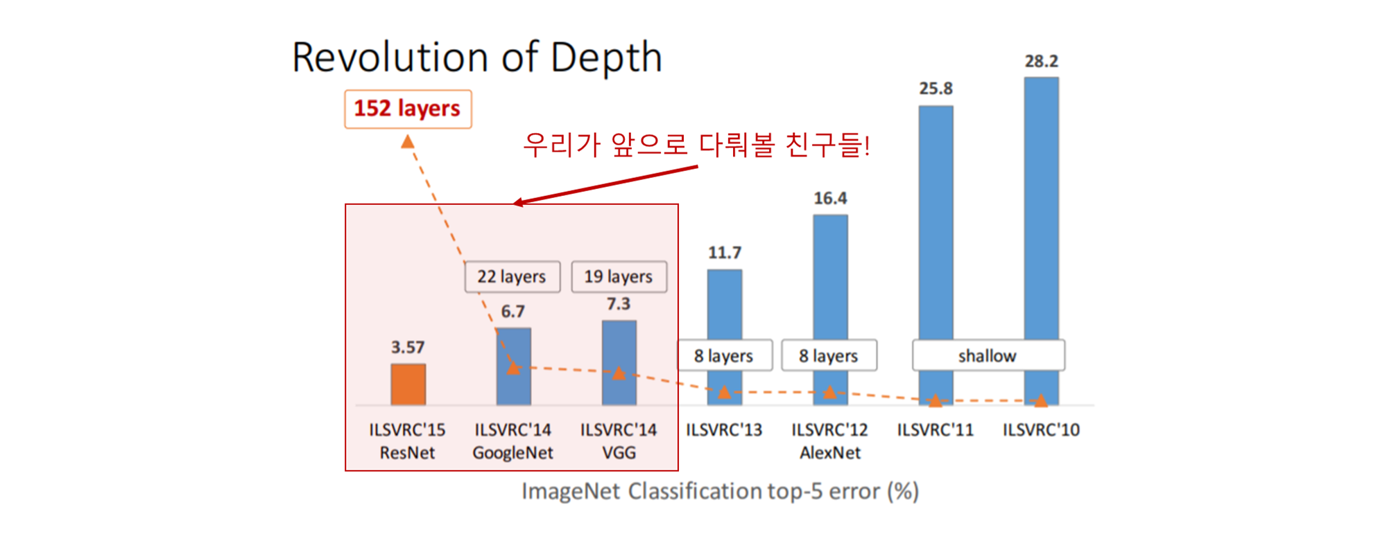
Source : https://icml.cc/2016/tutorials/
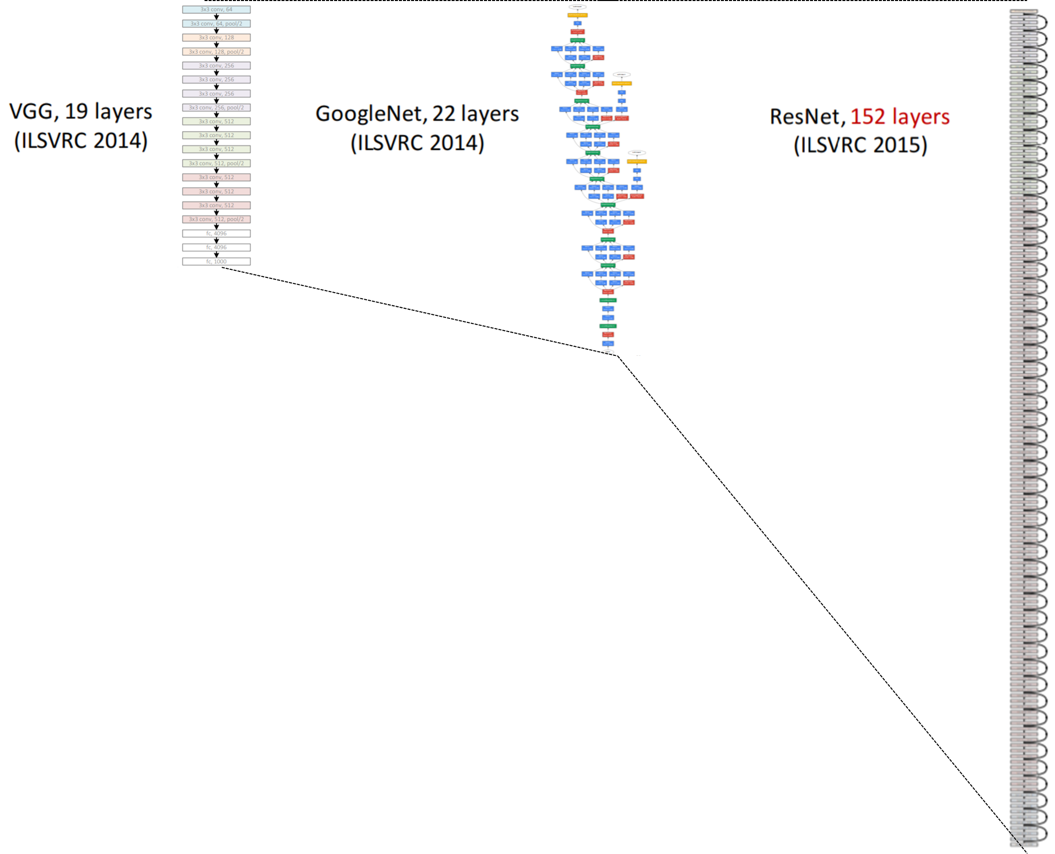
위의 그림에서 layers는 CNN layer의 개수(깊이)를 의미하며 직관적인 이해를 위해서 아래처럼 그림을 그려보았습니다.
ResNet 개요
소개
ResNet이 소개된 논문의 제목은 Going Deeper with Convolutions로, 다음 링크에서 확인해보실 수 있습니다. (링크)
ResNet의 저자들은 일정 수준 이상의 깊이가 되면 오히려 얕은 모델보다 깊은 모델의 성능이 더 떨어진다는 것을 아래 그림과 같이 확인할 수 있었습니다.
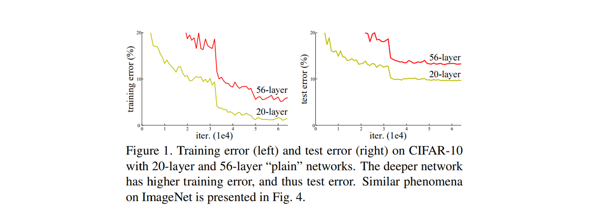
Plane network 20-layer와 56-layer의 train error와 test error (논문 발췌)
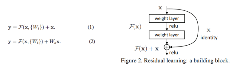
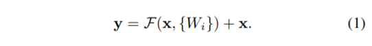
이러한 문제를 해결하기 위해 잔차 학습(residual learning)이라는 방법을 통해 모델 성능을 향상시킨 것이 바로 ResNet입니다. 아이디어는 정말 심플한데요. 특정 위치에서 입력이 들어왔을 때 합성곱 연산을 통과한 결과와 입력으로 들어온 결과 두가지를 더해서 다음 레이어에 전달하는 것이 ResNet의 핵심입니다. (아래 그림 참고)
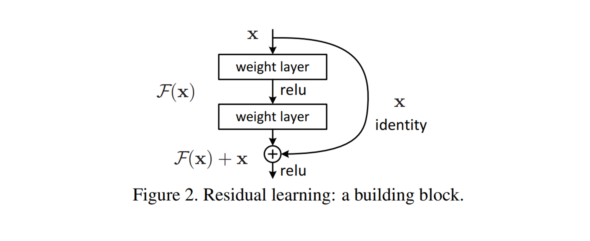
Residual Learning (논문 발췌)
위 그림에서 볼 수 있다시피 잔차 학습은 이전 단계에서 뽑았던 특성들을 변형시키지 않고, 그대로 다음 단계로 전달하여 더해주기 때문에 앞에서 학습한 low-level 특징과 뒤에서 학습한 high-level 특징을 모두 다음 block(단계)로 전달할 수 있다는 장점을 가지고 있습니다. 이전 GoogleNet의 경우, Neural Network의 Vanishing Gradient 문제를 해결하기 위해 Auxilary Classifier를 사용하였습니다. 하지만, ResNet의 경우 더하기 연산은 기울기가 1이기 때문에 역전파 시 loss가 줄지 않고, 모델 앞까지 잘 전파가 된다는 특징이 있어서 GoogleNet과는 다르게 Auxilary Classifier가 별도로 필요하지 않습니다.
모델 구조
Overall Network
논문에서는 VGG-19, 34-layer Plain (without residual) 모델과 34-layer Residual 모델을 다음과 같이 시각화하고 있습니다.

VGG-19, 34-layer Plain & Residual (논문 발췌)
위 그림에서 실선은 featuremap의 dimension이 바뀌지 않아 그냥 더해주는 경우이고, 점선은 입력단과 출력단의 dimension의 차이로 인해 이를 맞춰줄 수 있는 테크닉이 추가적으로 더해진 shortcut connection입니다.
아래표는 논문에서 제안하는 다양한 유형의 ResNet구조들입니다. 위 그림의 예시는 아래 그림에서 34-layer 모델과 동일합니다.
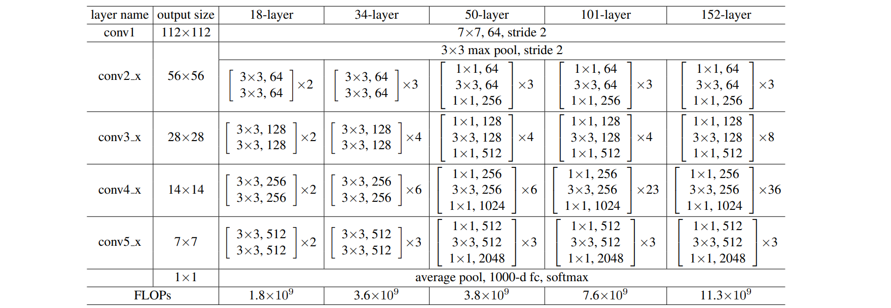
ResNet 19, 34, 50, 101, 152 layer
Plain Network
Plain Network은 다음과 같은 규칙에 따라 만들어졌습니다:
- 같은 크기의 output feature map을 갖고 있다면, 같은 수의 filters를 갖도록 합니다.
- 만약 feature map size가 반으로 줄어들었다면, time-complexity를 유지하기 위해 filters의 수는 두 배가 되도록 합니다.
- Downsampling을 하기 위해서 stride가 2인 conv layers를 통과시켜줍니다.
- 1x1 convolution의 경우, 동일한 사이즈의 feature map을 유지하기 위해 별도의 padding이 필요없습니다.
- 하지만, 3x3 convolution의 경우, 동일한 사이즈의 feature map을 유지하기 위해 size 1의 padding이 필요하게 됩니다.
- Network의 마지막 단에는 Global Average Pooling(GAP)를 수행하며, ImageNet Classification을 목적으로 하기 때문에 1000-way-fully-connected layer로 이루어져 있습니다.
Residual Network
Residual Network
Residual Network(ResNet)의 기본적인 조건은 위의 plain network와 동일합니다. 한가지 다른 점은 각각의 block들이 끝날때마다 shortcut connection 추가된다는 점입니다.
- input과 output의 차원이 같다면 identity shortcut은 바로 사용될 수 있습니다. (1)
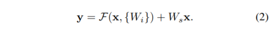
- 하지만, 차원이 다르다면 identity shortcut을 바로 사용할 수 없습니다. Identity Shortcut 대신 Projection Shortcut이 사용되게 됩니다. (By using 1x1 Convolution) (2)
Shortcuts Comparison
- 해당 논문에서는 shortcut의 사용방법에 따른 성능을 아래와 같이 비교합니다.
-
(A) Increasing Dimension에 Zero Padding을 활용한 Shortcut을 사용
-
(B) Increasing Dimension에 Projection Shortcut을 사용
-
(C) 모든 Shortcut을 Projection Shortcut으로 대체하여 사용
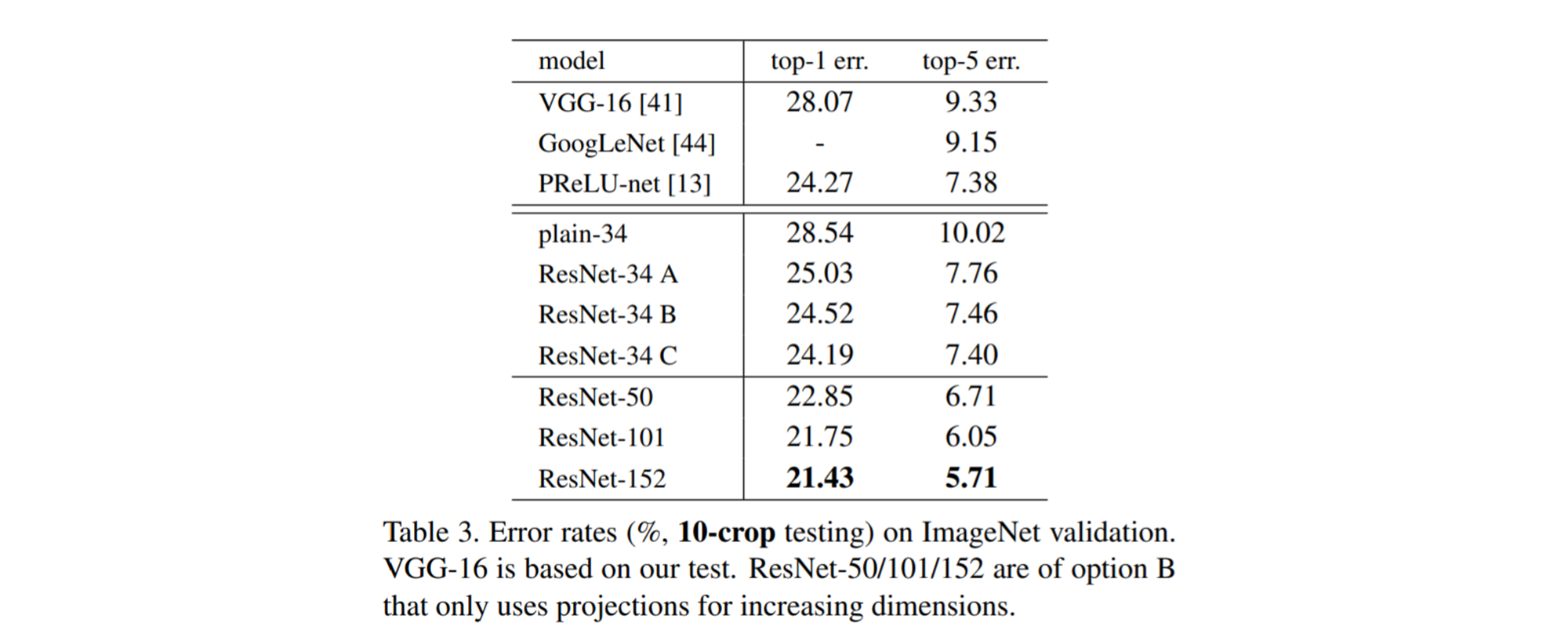
Table 3을 보면 3가지 옵션 모두 Plain Network보다 성능이 좋으며, A < B < C순으로 성능이 좋은 것을 확인할 수 있습니다. 논문에서는 B가 A보다 나은 이유를 A의 zero-padding과정에 residual learning이 없기 때문이라고 말합니다. 그리고, C가 B보다 좋은 이유로는 extra parameters가 더 많기 때문에 이는 성능 향상으로 이어졌다고 이야기 합니다.
A, B, C에서의 작은 차이를 통해 알 수 있는 것은 Projection Shortcut은 본 논문에서 문제 삼고 있는 degradation 문제를 address 하는 것의 본질이 아니라는 것을 보여줍니다. 또한, extra parameter가 추가되는 C는 memory & time complexity 를 줄이기 위해 사용되지 않았습니다.
Deeper Bottleneck Architecture
본 논문에서 저자들은 Layer 가 깊어지면 training time 이 증가하는 것을 발견하였고, 이를 고려하여 Residual Block을 아래와 같이 1x1 Convolution을 활용하여 개선한 Bottleneck Block을 제안하였습니다.

Bottleneck Block은 1x1, 3x3, 1x1 convolution으로 구성된 3개의 Layer를 쌓은 구조로, Basic Block 보다 Layer 수가 1개 더 많지만, time complexity는 비슷하다는 특징을 갖고 있습니다. 이때 Bottleneck Block에는 앞에서 소개한 옵션 B를 적용하였습니다.
이런 방법을 적용하여 깊은 모델(50-layer, 101-layer, 152-layer에 적용해본 결과, 기존의 degradation의 문제가 발생하지 않고, 깊이가 더 깊어짐에 따라 더 좋아지는 것을 확인할 수 있었습니다.
실험
CIFAR 10
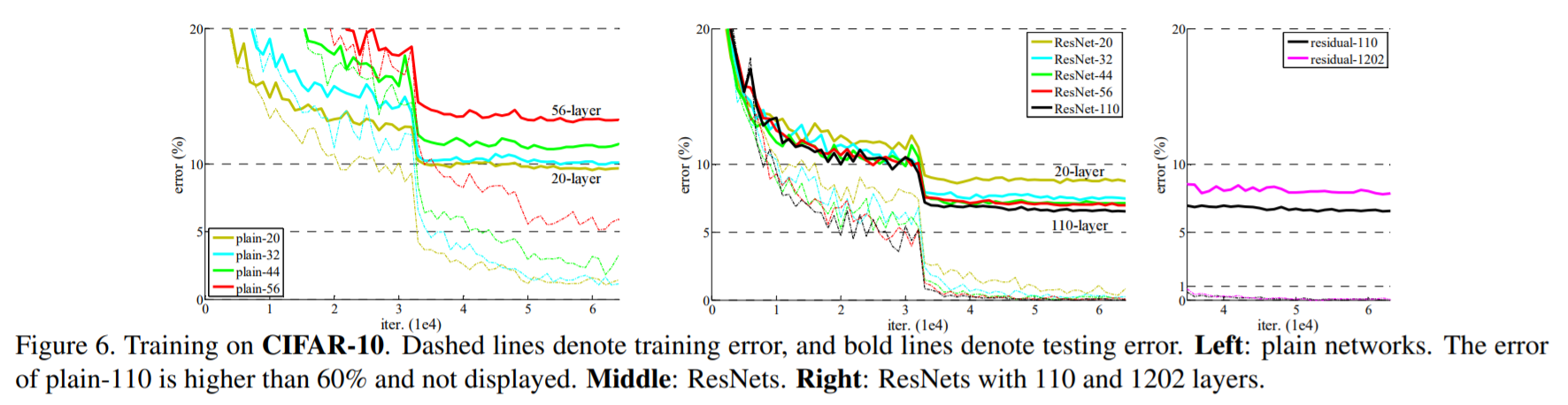
먼저 CIFAR10 데이터에 대하여 실험한 결과는 다음과 같습니다. 점선은 Training Error를 의미하고, 실선은 Test Error를 의미합니다.
-
Figure 6의 좌측에 있는 그래프는 residual 연산을 사용하지 않은 plain network를 사용했을 때의 Error입니다. 이를 살펴보면 layer가 깊을 수록 Error가 높은 것을 확인할 수 있습니다. (Degradation 문제)
-
Figure 6의 중앙에 있는 그래프는 residual 연산을 사용한 residual network를 사용했을 때의 Error입니다. 이를 살펴보면 layer가 깊을 수록 Error가 낮은 것을 확인할 수 있습니다.
-
Figure 6의 우측에 있는 그래프는 1202-layer residual network와 110-layer residual network로, 유사한 training error 보였지만 test 성능은 더 좋지 않은 것으로 보아 Overfitting이 발생한 것을 확인할 수 있었습니다.
PASCAL VOC & MS COCO
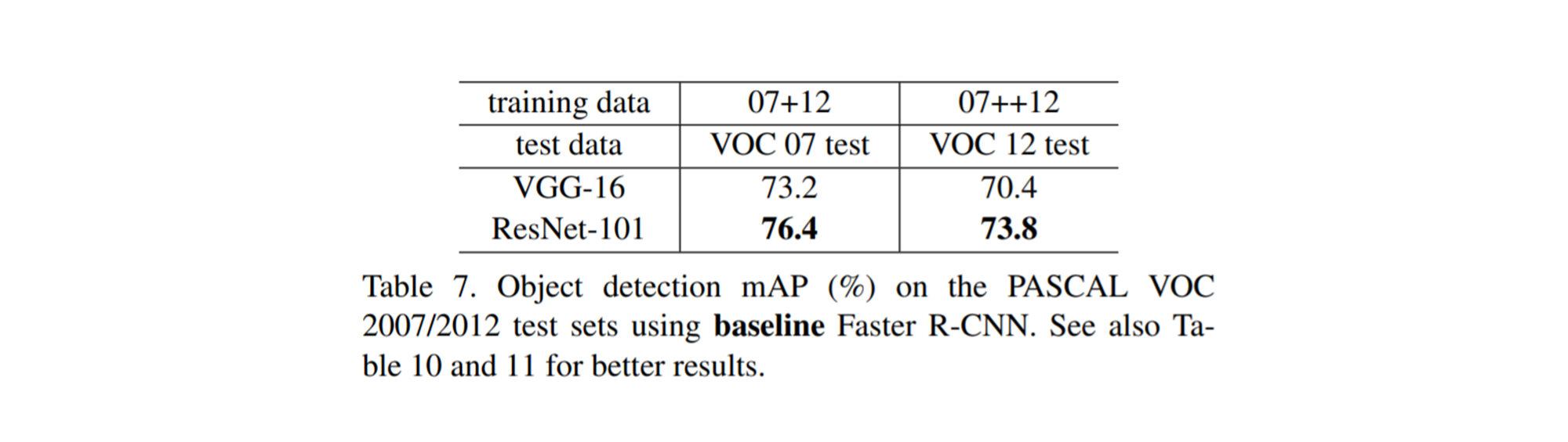
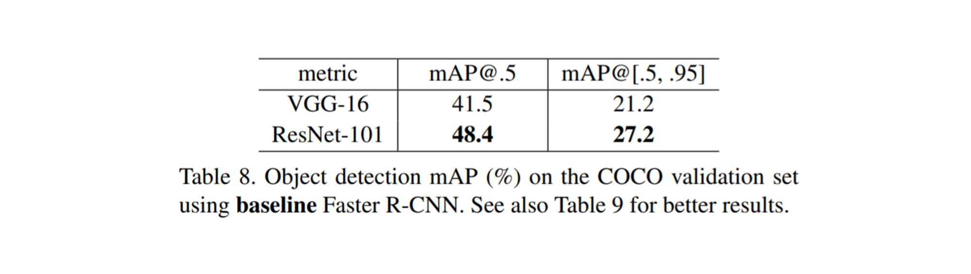
각각 PASCAL VOC 2007/2012 데이터와 MS COCO 데이터를 사용한 Object Detection에 있어서도 VGGNet을 사용한 것보다 ResNet을 사용한 것이 더 좋은 성능이 나오는 것을 확인할 수 있습니다.
PASCAL VOC 2007/2012
MS COCO
코드
이번 포스트에서는 ResNet-50을 구현해보는 시간을 갖겠습니다.
라이브러리
import torch
import torch.nn as nn
import torch.optim as optim
import torch.nn.init as init

import torchvision
import torchvision.datasets as datasets
import torchvision.transforms as transforms

from torch.utils.data import DataLoader

import numpy as np
import matplotlib.pyplot as plt

import tqdm
from tqdm.auto import trange
하이퍼파라미터
batch_size = 50
learning_rate = 0.0002
num_epoch = 100
Load CIFAR-10
transform = transforms.Compose([transforms.ToTensor(), transforms.Normalize((0.5, 0.5, 0.5), (0.5, 0.5, 0.5))])

# define dataset
cifar10_train = datasets.CIFAR10(root="../Data/", train=True, transform=transform, target_transform=None, download=True)
cifar10_test = datasets.CIFAR10(root="../Data/", train=False, transform=transform, target_transform=None, download=True)

# define loader
train_loader = DataLoader(cifar10_train,batch_size=batch_size, shuffle=True, num_workers=2, drop_last=True)
test_loader = DataLoader(cifar10_test,batch_size=batch_size, shuffle=False, num_workers=2, drop_last=True)

# define classes
classes = ('plane', 'car', 'bird', 'cat', 'deer', 'dog', 'frog', 'horse', 'ship', 'truck')
Basic Module
def conv_block_1(in_dim,out_dim, activation,stride=1):
    model = nn.Sequential(
        nn.Conv2d(in_dim,out_dim, kernel_size=1, stride=stride),
        nn.BatchNorm2d(out_dim),
        activation,
    )
    return model


def conv_block_3(in_dim,out_dim, activation, stride=1):
    model = nn.Sequential(
        nn.Conv2d(in_dim,out_dim, kernel_size=3, stride=stride, padding=1),
        nn.BatchNorm2d(out_dim),
        activation,
    )
    return model
Bottleneck Module
class BottleNeck(nn.Module):
    def __init__(self,in_dim,mid_dim,out_dim,activation,down=False):
        super(BottleNeck,self).__init__()
        self.down=down

        # 특성지도의 크기가 감소하는 경우
        if self.down:
            self.layer = nn.Sequential(
              conv_block_1(in_dim,mid_dim,activation,stride=2),
              conv_block_3(mid_dim,mid_dim,activation,stride=1),
              conv_block_1(mid_dim,out_dim,activation,stride=1),
            )

            # 특성지도 크기 + 채널을 맞춰주는 부분
            self.downsample = nn.Conv2d(in_dim,out_dim,kernel_size=1,stride=2)

        # 특성지도의 크기가 그대로인 경우
        else:
            self.layer = nn.Sequential(
                conv_block_1(in_dim,mid_dim,activation,stride=1),
                conv_block_3(mid_dim,mid_dim,activation,stride=1),
                conv_block_1(mid_dim,out_dim,activation,stride=1),
            )

        # 채널을 맞춰주는 부분
        self.dim_equalizer = nn.Conv2d(in_dim,out_dim,kernel_size=1)

    def forward(self,x):
        if self.down:
            downsample = self.downsample(x)
            out = self.layer(x)
            out = out + downsample
        else:
            out = self.layer(x)
            if x.size() is not out.size():
                x = self.dim_equalizer(x)
            out = out + x
        return out
Define ResNet-50
# 50-layer
class ResNet(nn.Module):

    def __init__(self, base_dim, num_classes=10):
        super(ResNet, self).__init__()
        self.activation = nn.ReLU()
        self.layer_1 = nn.Sequential(
            nn.Conv2d(3,base_dim,7,2,3),
            nn.ReLU(),
            nn.MaxPool2d(3,2,1),
        )
        self.layer_2 = nn.Sequential(
            BottleNeck(base_dim,base_dim,base_dim*4,self.activation),
            BottleNeck(base_dim*4,base_dim,base_dim*4,self.activation),
            BottleNeck(base_dim*4,base_dim,base_dim*4,self.activation,down=True),
        )
        self.layer_3 = nn.Sequential(
            BottleNeck(base_dim*4,base_dim*2,base_dim*8,self.activation),
            BottleNeck(base_dim*8,base_dim*2,base_dim*8,self.activation),
            BottleNeck(base_dim*8,base_dim*2,base_dim*8,self.activation),
            BottleNeck(base_dim*8,base_dim*2,base_dim*8,self.activation,down=True),
        )
        self.layer_4 = nn.Sequential(
            BottleNeck(base_dim*8,base_dim*4,base_dim*16,self.activation),
            BottleNeck(base_dim*16,base_dim*4,base_dim*16,self.activation),
            BottleNeck(base_dim*16,base_dim*4,base_dim*16,self.activation),
            BottleNeck(base_dim*16,base_dim*4,base_dim*16,self.activation),
            BottleNeck(base_dim*16,base_dim*4,base_dim*16,self.activation),
            BottleNeck(base_dim*16,base_dim*4,base_dim*16,self.activation,down=True),
        )
        self.layer_5 = nn.Sequential(
            BottleNeck(base_dim*16,base_dim*8,base_dim*32,self.activation),
            BottleNeck(base_dim*32,base_dim*8,base_dim*32,self.activation),
            BottleNeck(base_dim*32,base_dim*8,base_dim*32,self.activation),
        )
        self.avgpool = nn.AvgPool2d(1,1)
        self.fc_layer = nn.Linear(base_dim*32,num_classes)

    def forward(self, x):
        out = self.layer_1(x)
        out = self.layer_2(out)
        out = self.layer_3(out)
        out = self.layer_4(out)
        out = self.layer_5(out)
        out = self.avgpool(out)
        out = out.view(batch_size,-1)
        out = self.fc_layer(out)

        return out
Train
device = torch.device("cuda:0")
model = ResNet(base_dim=64).to(device)
loss_func = nn.CrossEntropyLoss()
optimizer = optim.Adam(model.parameters(),lr=learning_rate)

loss_arr = []
for i in trange(num_epoch):
    for j,[image,label] in enumerate(train_loader):
        x = image.to(device)
        y_= label.to(device)

        optimizer.zero_grad()
        output = model.forward(x)
        loss = loss_func(output,y_)
        loss.backward()
        optimizer.step()

    if i % 10 ==0:
        print(loss)
        loss_arr.append(loss.cpu().detach().numpy())
성능 (epoch = 100)
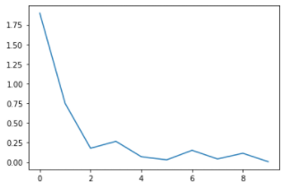
Train Loss
Test Accuracy
Accuracy of Test Data: 74.33999633789062%