(221004) 컨볼루션 신경망 모델 이용하여 이미지 분석 및 예측하기

1. 컨볼루션 신경망 모델 이용하여 Fashion_MNIST 다중 분류하기

1) 문제 정의

• 10가지 의류(0-9)를 예측하는 다중분류 문제

2) Fashion_MNIST 데이터 준비하기

from keras.datasets.fashion_mnist import load_data

# keras 저장소에서 데이터 다운로드
(X_train, y_train), (X_test, y_test) = load_data()
print(X_train.shape, X_test.shape)

3) 데이터 그려보기

import matplotlib.pyplot as plt
import numpy as np
np.random.seed(777)

class_names = ['T-shirt/top', 'Trouser', 'Pullover', 'Dress', 'Coat',
               'Sandal', 'Shirt', 'Sneakers', 'Bag', 'Ankle boots']

sample_size = 9 # 9개 뽑아줘
random_idx = np.random.randint(60000, size=sample_size)  # 6만개 중 9개 랜덤하게 보여줘

plt.figure(figsize=(5,5))
for i, idx in enumerate(random_idx):
  plt.subplot(3,3,i+1)
  plt.xticks([]) # 안 그릴거라 비우기
  plt.yticks([])
  plt.imshow(X_train[idx], cmap ='gray')
  plt.xlabel(class_names[y_train[idx]])
plt.show()

4) 전처리 및 검증 데이터셋 만들기

# 1) X feature의 값을  0-1 구간으로 정규화; MinMax 알고리즘 사용해 스케일링
# 2) Cov2D 신경망 사용하기 위해 3채원 배열으로 변환

X_train = np.reshape(X_train / 255, (-1, 28, 28, 1)) 
# -1: 개수가 맞지 않아도 오류내지 말고 reshape 해줘
X_test = np.reshape(X_test / 255, (-1, 28, 28, 1))

X_train.shape

• 결과값: (60000, 28, 28, 1)
• 컨볼루션 신경망은 3차원으로 받길 원함(기존 2차원 이미지 + 컬러값) -> 2차원에서 3차원으로 변경시켜줘야 함
• 현재는 (60000, 28, 28)으로 60000개의 데이터가 28*28의 형태로 존재
• 3차원 배열 = (width, height, color) color 1 = 흑백, color 3 = 컬러 예시.(28,28,1)

# 3) 각 레이블을 범주형으로 변경
# 현재: 0-9 -> 변경 후: [1,0,0,0,0,0,0,0,0,0] (원핫 인코딩)

from tensorflow.keras.utils import to_categorical
y_train = to_categorical(y_train)
y_test = to_categorical(y_test)

y_test

• 결과값: array([[0., 0., 0., ..., 0., 0., 1.],
  [0., 0., 1., ..., 0., 0., 0.],
  [0., 1., 0., ..., 0., 0., 0.],
  ...,
  [0., 0., 0., ..., 0., 1., 0.],
  [0., 1., 0., ..., 0., 0., 0.],
  [0., 0., 0., ..., 0., 0., 0.]], dtype=float32)
  

# 4) 검증 데이터 셋 분리; 훈련 -> 훈련 70 :  검증 30 

from sklearn.model_selection import train_test_split

X_train, X_val, y_train, y_val = train_test_split(X_train, y_train, test_size=0.3, 
                                                  random_state=777)

print(X_train.shape) 
print(X_val.shape) 

• 결과값:
  (42000, 28, 28, 1)
  (18000, 28, 28, 1)

5) 컨볼루션 신경망 모델 구성하기

from tensorflow.keras.models import Sequential
from tensorflow.keras.layers import Conv2D, MaxPool2D, Dense, Flatten

model = Sequential()
model.add(Conv2D(filters=16, kernel_size=3, strides=(1,1), padding='same', 
                 activation='relu', input_shape=(28,28,1)))       
               
model.add(MaxPool2D(pool_size=(2,2), strides=2, padding='same'))
# 2*2로 지나가면서 특징 추출하고 Max값으로 다운 샘플링해줄 것이다. -> (14, 14, 1)
model.add(Conv2D(filters=32, kernel_size=3, strides=(1,1), padding='same', 
                 activation='relu'))
model.add(MaxPool2D(pool_size=(2,2), strides=2, padding='same')) # -> (7, 7, 1)     
model.add(Conv2D(filters=64, kernel_size=3, strides=(1,1), padding='same', 
                 activation='relu'))
model.add(MaxPool2D(pool_size=(2,2), strides=2, padding='same')) # -> (4, 4, 1)   
model.add(Flatten()) # 2차원 배열을 Dense층에 입력하기 위해 1차원으로 펼침
model.add(Dense(64, activation ='relu'))
model.add(Dense(10, activation ='softmax')) # 10개의 출력을 가진 신경망

• kernel_size=3 : 3x3 필터 사이즈 사용
• stride=1 : 한칸씩 움직이면서 스트라이드 (특징맵 추출)
• padding 기본값은 'valid'로 사용하지 않겠다고 설정되어 있음

6) 컨볼루션 신경망 모델 확인하기

from tensorflow.keras.utils import plot_model
plot_model(model, 'model.png', show_shapes=True)

model.summary()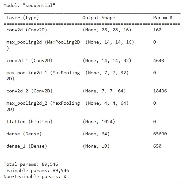

7) 모델 설정 및 학습하기

model.compile(optimizer='adam', loss='categorical_crossentropy', metrics=['acc'])

history = model.fit(X_train, y_train, epochs=30, 
                    batch_size=32, validation_data=(X_val, y_val))

8) 학습결과 그리기

import matplotlib.pyplot as plt

his_dict = history.history
loss = his_dict['loss']
val_loss = his_dict['val_loss'] # 검증 데이터가 있는 경우 ‘val_’ 수식어가 붙습니다. # 추가

epochs = range(1, len(loss) + 1)
fig = plt.figure(figsize = (10, 5))

# 훈련 및 검증 손실 그리기
ax1 = fig.add_subplot(1, 2, 1)
ax1.plot(epochs, loss, color = 'blue', label = 'train_loss')
ax1.plot(epochs, val_loss, color = 'orange', label = 'val_loss') # 추가
ax1.set_title('train and val loss') 
ax1.set_xlabel('epochs')
ax1.set_ylabel('loss')
ax1.legend()

acc = his_dict['acc']
val_acc = his_dict['val_acc'] # 추가

# 훈련 및 검증 정확도 그리기
ax2 = fig.add_subplot(1, 2, 2)
ax2.plot(epochs, acc, color = 'blue', label = 'train_acc')
ax2.plot(epochs, val_acc, color = 'orange', label = 'val_acc') # 추가
ax2.set_title('train and val acc')
ax2.set_xlabel('epochs')
ax2.set_ylabel('loss')
ax2.legend()

plt.show()

• 과대적합되어 있는 상태
• 가중치 조정이 잘못 되어가고 있다.
• 학습횟수를 5번으로 줄이는 것이 좋겠다라는 판단. -> 5번으로 일반화된 모델을 만드는 것이 좋다.

9) 모델 평가하기

model.evaluate(X_test, y_test)

• 결과값: 313/313 - 1s 3ms/step - loss: 0.5309 - acc: 0.9084
  
  
  
  

2. 컨볼루션 신경망(CNN) 모델 이용하여 개/고양이 이미지 분류하기

1) 문제정의

• 개(1), 고양이(0) 이미지를 예측하는 이진분류 문제

2) 데이터 준비하기

• 코랩 이용 - google api를 통해 데이터 불러오기

!wget --no-check-certificate \
    https://storage.googleapis.com/mledu-datasets/cats_and_dogs_filtered.zip \
    -O /tmp/cats_and_dogs_filtered.zip

• tmp에 저장된 파일 확인가능

3) 데이터 폴더 나누기

# 압축풀기
import os
import zipfile

local_zip = '/tmp/cats_and_dogs_filtered.zip'
zip_ref = zipfile.ZipFile(local_zip, 'r') # 'r' = 읽기
zip_ref.extractall('/tmp')
zip_ref.close()

# 데이터 경로 설정
rootPath = '/tmp/cats_and_dogs_filtered' # 기본 경로

# 훈련 및 검증 데이터 경로
train_dir = os.path.join(rootPath, 'train') 
# 운영체제에서 제공해주는 경로를 붙이는 함수 join -> /tmp/cats_and_dogs_filtered/train
val_dir = os.path.join(rootPath, 'validation') 
# -> /tmp/cats_and_dogs_filtered/validation

# 훈련 데이터 중 고양이 사진 경로
train_cats_dir = os.path.join(train_dir, 'cats') 
# -> /tmp/cats_and_dogs_filtered/train/cats
# 훈련 데이터 중 강아지 사진 경로
train_dogs_dir = os.path.join(train_dir, 'dogs') 
# -> /tmp/cats_and_dogs_filtered/train/dogs

# 검증 데이터 중 고양이 사진 경로
val_cats_dir = os.path.join(val_dir, 'cats') 
# -> /tmp/cats_and_dogs_filtered/validation/cats
# 검증 데이터 중 강아지 사진 경로
val_dogs_dir = os.path.join(val_dir, 'dogs') 
# -> /tmp/cats_and_dogs_filtered/validation/dogs

4) 데이터 확인하기

train_cat_fnames = os.listdir(train_cats_dir)
train_cat_fnames.sort()
train_dog_fnames = os.listdir(train_dogs_dir)
train_dog_fnames.sort()
val_cat_fnames = os.listdir(val_cats_dir)
val_cat_fnames.sort()
val_dog_fnames = os.listdir(val_dogs_dir)
val_dog_fnames.sort()

# print(train_dog_fnames[:10])

print('훈련 고양이 데이터 사진 수: ', len(os.listdir(train_cats_dir)))
print('훈련 강아지 데이터 사진 수: ', len(os.listdir(train_dogs_dir)))
print('검증 고양이 데이터 사진 수: ', len(os.listdir(val_cats_dir)))
print('검증 강아지 데이터 사진 수: ', len(os.listdir(val_dogs_dir)))

• 결과값:
  훈련 고양이 데이터 사진 수: 1000
  훈련 강아지 데이터 사진 수: 1000
  검증 고양이 데이터 사진 수: 500
  검증 강아지 데이터 사진 수: 500

5) 데이터 증식(Data Augmentation)

import os
from tensorflow.keras.preprocessing.image import ImageDataGenerator

# 데이터 경로 설정
rootPath = '/tmp/cats_and_dogs_filtered'

# 각 데이터의 generate를 개별적으로 진행
# 훈련 데이터는 데이터 증식(속성) + 정규화(스케일링)
trainImageGenerator = ImageDataGenerator(rescale=1./255,
                                         horizontal_flip = True,
                                         vertical_flip = True,
                                         shear_range = 0.5,
                                         brightness_range = [0.5, 1.5],
                                         zoom_range = 0.2,
                                         width_shift_range = 0.1,
                                         height_shift_range = 0.1,
                                         rotation_range = 30,
                                         fill_mode = 'nearest')
# 검증 데이터는 정규화만(스케일링) 
testImageGenerator = ImageDataGenerator(rescale=1./255)

trainGen = trainImageGenerator.flow_from_directory(
    os.path.join(rootPath, 'train'),
    target_size = (64, 64),
    class_mode = 'binary') # 0과 1로 라벨링을 하고 데이터를 읽어들임

testGen = testImageGenerator.flow_from_directory(
    os.path.join(rootPath, 'validation'),
    target_size = (64, 64),
    class_mode = 'binary') # categorical로 주면 다중 분류 가능

• 이미지제너레이터를 활용하여 데이터를 증식하는 속성은 여러가지가 있다.
• 수평 및 수직 반전, 밝기, 확대, 좌우 및 상하 이동, 각도 회전 등
• 이렇게 데이터를 증식하더라도 기본적인 공간 속성은 변하지 않는다는 것이 전제

# 라벨 확인
print(trainGen.class_indices) 
print(testGen.class_indices)

• 딕셔너리 형태 key: 개, 고양이 value: 1, 0

# 훈련 데이터 그려보기
from tensorflow.keras.preprocessing.image import array_to_img
import matplotlib.pyplot as plt
import numpy as np

plt.figure(figsize=(5,5))

for i in range(9):
  data = next(trainGen)
  arr = data[0][0]
  plt.subplot(3, 3, i+1)
  plt.xticks([]) #눈금 지우기 코드
  plt.yticks([])
  img = array_to_img(arr).resize((128,128))
  plt.imshow(img)

plt.show()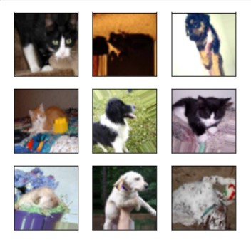

• 정규화와 이미지 증식이 모두 이루어진 모습을 확인할 수 있다.

# 검증 데이터 그려보기
from tensorflow.keras.preprocessing.image import array_to_img
import matplotlib.pyplot as plt
import numpy as np

plt.figure(figsize=(5,5))

for i in range(9):
  data = next(testGen)
  arr = data[0][0]
  plt.subplot(3, 3, i+1)
  plt.xticks([]) #눈금 지우기 코드
  plt.yticks([])
  img = array_to_img(arr).resize((128,128))
  plt.imshow(img)

plt.show()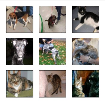

• 정규화만 처리했기 때문에 이미지 변화가 없는 모습이다.(좌우상하 반전 등)

# 정답지 그려보기
label_index = trainGen.class_indices

x,y = trainGen.next()

# print(len(x)) # next는 32개씩 줌
for i in range(0,3):
  image = x[i]
  label = y[i].astype('int')
  plt.xticks([]) #눈금 지우기 코드
  plt.yticks([])
  print('사진: {}'.format([k for k, v in label_index.items() if v == label])) 
  # {'cats': 0, 'dogs': 1} -> {0 : 'cats', 1 : 'dogs'} 이름으로 보여주도록 코딩
  print('사진: {}'.format(label)) # 원래 출력 데이터
  plt.imshow(image)
  plt.show()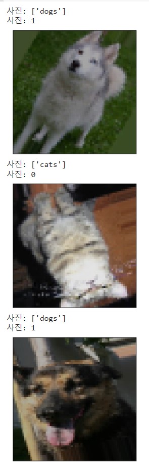

6) 간단한 CNN 모델 구성하기

from tensorflow.keras.models import Sequential
from tensorflow.keras import layers

model = Sequential()

model.add(layers.InputLayer(input_shape=(64, 64, 3)))
model.add(layers.Conv2D(16, (3,3), (1,1), 'same', activation = 'relu')) 
# 필터 사이즈, 커널 사이즈, 스트라이드, 패딩 여부, 활성화 함수 순
model.add(layers.MaxPooling2D((2,2)))
model.add(layers.Dropout(rate=0.3))

model.add(layers.Conv2D(32, (3,3), (1,1), 'same', activation = 'relu')) 
# 필터 사이즈, 커널 사이즈, 스트라이드, 패딩 여부, 활성화 함수 순
model.add(layers.MaxPooling2D((2,2)))
model.add(layers.Dropout(rate=0.3))

model.add(layers.Conv2D(64, (3,3), (1,1), 'same', activation = 'relu')) 
# 필터 사이즈, 커널 사이즈, 스트라이드, 패딩 여부, 활성화 함수 순
model.add(layers.MaxPooling2D((2,2)))
model.add(layers.Dropout(rate=0.3))

model.add(layers.Flatten())
model.add(layers.Dense(512, activation='relu'))
model.add(layers.Dense(256, activation='relu'))
model.add(layers.Dense(1, activation='sigmoid'))

7) 모델 그리기

from tensorflow.keras.utils import plot_model
plot_model(model, 'model.png', show_shapes=True)

model.summary()

8) 모델 설정 및 학습하기

model.compile(optimizer='adam', loss='binary_crossentropy', metrics=['acc'])

history = model.fit_generator(trainGen, epochs=32, validation_data = testGen) 

• testGen 안에 정답이 포함되어 있어서 문제지와 정답지 구분없이 통째로 넣어도 알아서 처리

9) 모델 학습결과 그리기

import matplotlib.pyplot as plt

his_dict = history.history
loss = his_dict['loss']
val_loss = his_dict['val_loss'] # 검증 데이터가 있는 경우 ‘val_’ 수식어가 붙습니다. # 추가

epochs = range(1, len(loss) + 1)
fig = plt.figure(figsize = (10, 5))

# 훈련 및 검증 손실 그리기
ax1 = fig.add_subplot(1, 2, 1)
ax1.plot(epochs, loss, color = 'blue', label = 'train_loss')
ax1.plot(epochs, val_loss, color = 'orange', label = 'val_loss') # 추가
ax1.set_title('train and val loss') 
ax1.set_xlabel('epochs')
ax1.set_ylabel('loss')
ax1.legend()

acc = his_dict['acc']
val_acc = his_dict['val_acc'] # 추가

# 훈련 및 검증 정확도 그리기
ax2 = fig.add_subplot(1, 2, 2)
ax2.plot(epochs, acc, color = 'blue', label = 'train_acc')
ax2.plot(epochs, val_acc, color = 'orange', label = 'val_acc') # 추가
ax2.set_title('train and val acc')
ax2.set_xlabel('epochs')
ax2.set_ylabel('loss')
ax2.legend()

plt.show()

10) 모델 평가하기

model.evaluate_generator(testGen)

• 결과값: [0.585421621799469, 0.6909999847412109]
• 정확도가 낮으니, 1) 맥스풀링을 최소화 하든, 2) 학습 횟수를 늘리든, 3) Dense 개수를 점진적으로 줄이든 다양한 방법을 사용하여 효율을 높일 수 있다.

11) 모델 예측하기

from tensorflow.keras.preprocessing.image import array_to_img
import numpy as np

label_index = ['고양이', '강아지']

x, y = testGen.next()

for i in range(0, 10):
  image = x[i]
  label = y[i].astype('int')

  y_prob = model.predict(image.reshape(1, 64, 64, 3))

  y_prob_class = (model.predict(image.reshape(1, 64, 64, 3)) > 0.5).astype('int')[0][0]
  print('정답: {}'.format(label_index[label]), ' label : ', label)
  print('예측: {}'.format(label_index[y_prob_class]), 'predicted value : ', y_prob)
  plt.imshow(image)
  plt.show()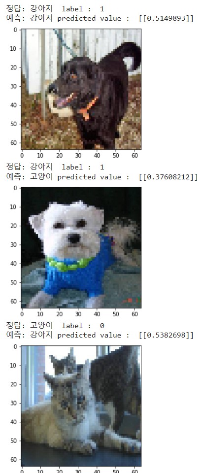

• 예측 정확도가 상당히 떨어짐을 한 번 더 확인 가능
• y prob에는 수치값(0-1 구간의 값)이 포함되어 있다
• T/F를 int형으로 변경하면, False = 0 , True = 1이 된다.

12) 학습횟수 변경하여 학습 후 모델 평가하기

history = model.fit_generator(trainGen, epochs=64, validation_data = testGen) 

model.evaluate_generator(testGen)

• 결과값: [0.5536543130874634, 0.7179999947547913]

참고. 검증 데이터는 원칙적으로 테스트 데이터와 달라야 하는데 우리는 이미지 데이터 분리 단계를 스킵했기 때문에 그냥 두 목적에 동일한 데이터를 중복 사용함.