Function Approximation: Pred

앞으로 계속 나오는 $v_{\pi}(s, w)$는 sample return을 의미한다

2.1) Policy evaluation을 위한 mse의 objective 이해하기

Mean Squared Value Error Objective

MSVEO를 최소화하기 위한 weight $\mu$를 찾자
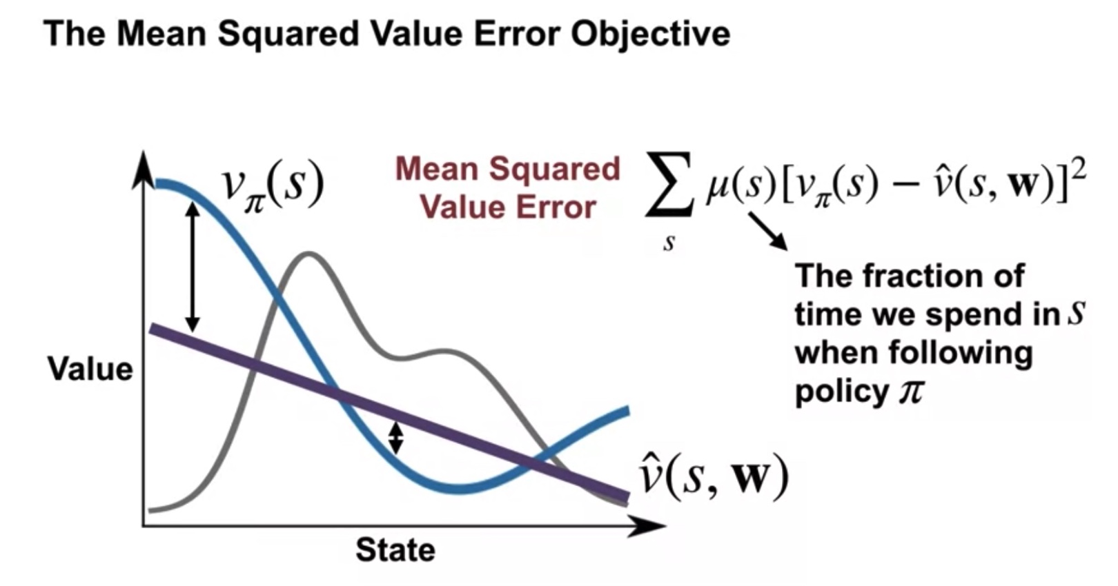Gray line is $\mu(s)$, weight

미지수 항

• $v_{\pi}(s)$ == True value function
• $\hat v(s,w)$ == Estimated value function
• $\mu(s)$ == Fraction(weight) of time we spend in $S_i$ following policy $\pi$

공식

• Mean Squared Value Error $\overline{VE}= \Sigma_s \mu(s) [v_{\pi}(s) - \hat v(s,w)]^2$

2.2) Gradient Monte for Policy evaluation

2.2.1. Gradient of the Mean Squared Value Error Objective

$\nabla \Sigma_s \mu(s) [v_{\pi}(s) - \hat v(s,w)]^2$

$= \Sigma_s \mu(s) \nabla [v_{\pi}(s) - \hat v(s,w)]^2$

$= -\Sigma_s \mu(s) 2[v_{\pi}(s) - \hat v(s,w)] \nabla(\hat v(s,w))$

저번 수업과의 차이점은...

• $\hat v(s,w) := \ <w,x(s)>$ : linear gradient approxi function에서 기울기 함수
• $\nabla \hat v(s,w) = x(s)$ : value function의 기울기 함수

2.2.2. Gradient Monte Carlo

MC에서는 중간의 추정값이 마지막까지 계산한 goal을 기준으로 갱신하기에
식을 다음과 같이 치환할 수 있다.
($\alpha$ == step size)

• 치환 전 $w_{t+1} := w_t + \alpha [v_{\pi}(S_t) - \hat v(S_t,w_t))] \nabla \hat v(S_t,w_t))$
• 치환 후 $w_{t+1} := w_t + \alpha [G_t - \hat v(S_t,w_t))] \nabla \hat v(S_t,w_t))$

이 때 $v_{\pi}(s) := E_{\pi}[G_t|S_t=s]$ 임을 고려하여
expectation gradient는 다음과 같이 치환할 수 있다.

• $E_{\pi}[2[v_{\pi}(S_t) - \hat v(S_t,w)]\nabla \hat v(S_t,w)]$
• = $E_{\pi}[2[G_t - \hat v(S_t,w)]\nabla \hat v(S_t,w)]$

여기까지 MC에 Stochastic Gradient Descent을 적용하는 법을 보였다.

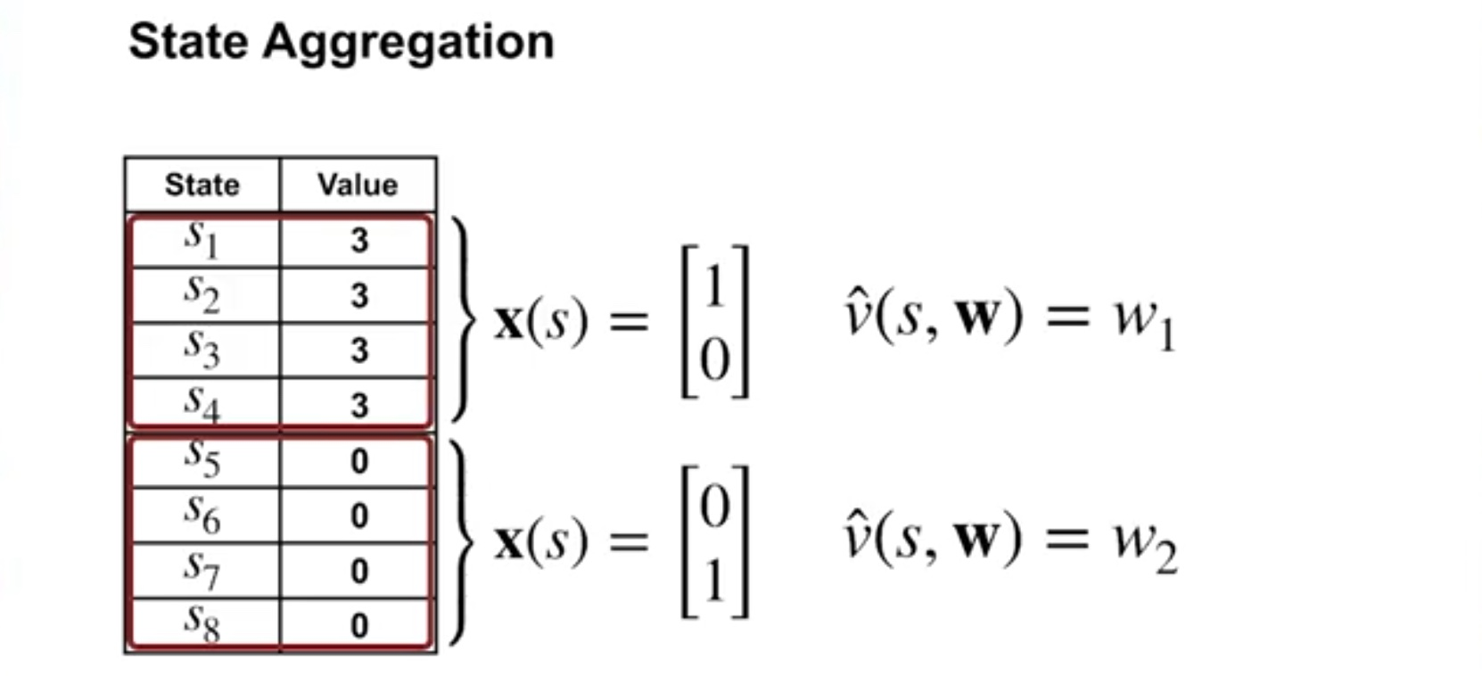
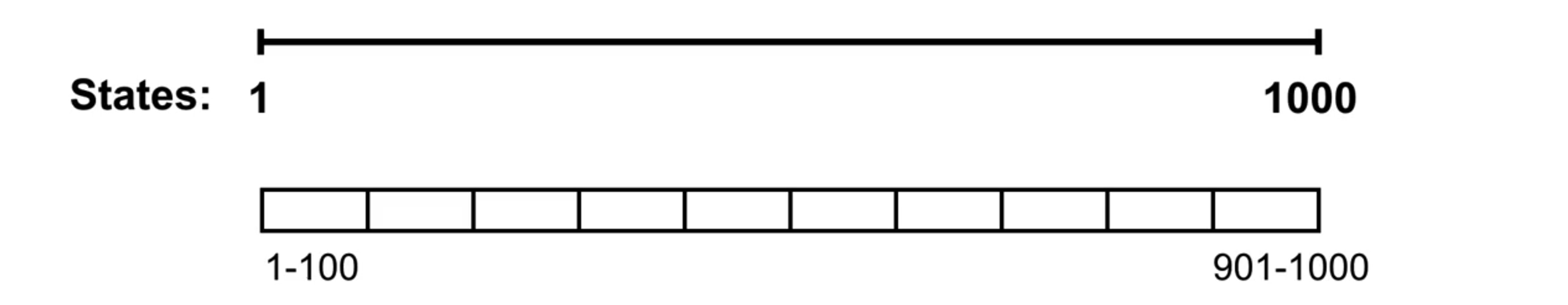
2.2.3 State Aggregation with Monte Carlo

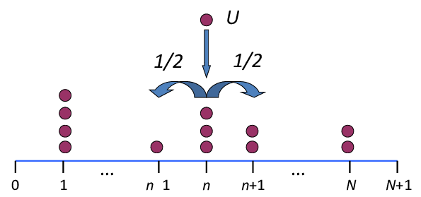
Random Walk Example

정중앙에서 시작해서 양쪽 끝으로 가면 도착인 문제
행동은 좌우로 각 50% 확률을 가진다.

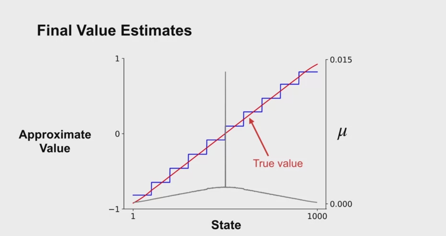
각 상태별로 가지는 value 값을 적어보고
같은 값을 가지는 상태끼리 그룹화를 하는 식으로 aggregation을 할 수 있다.

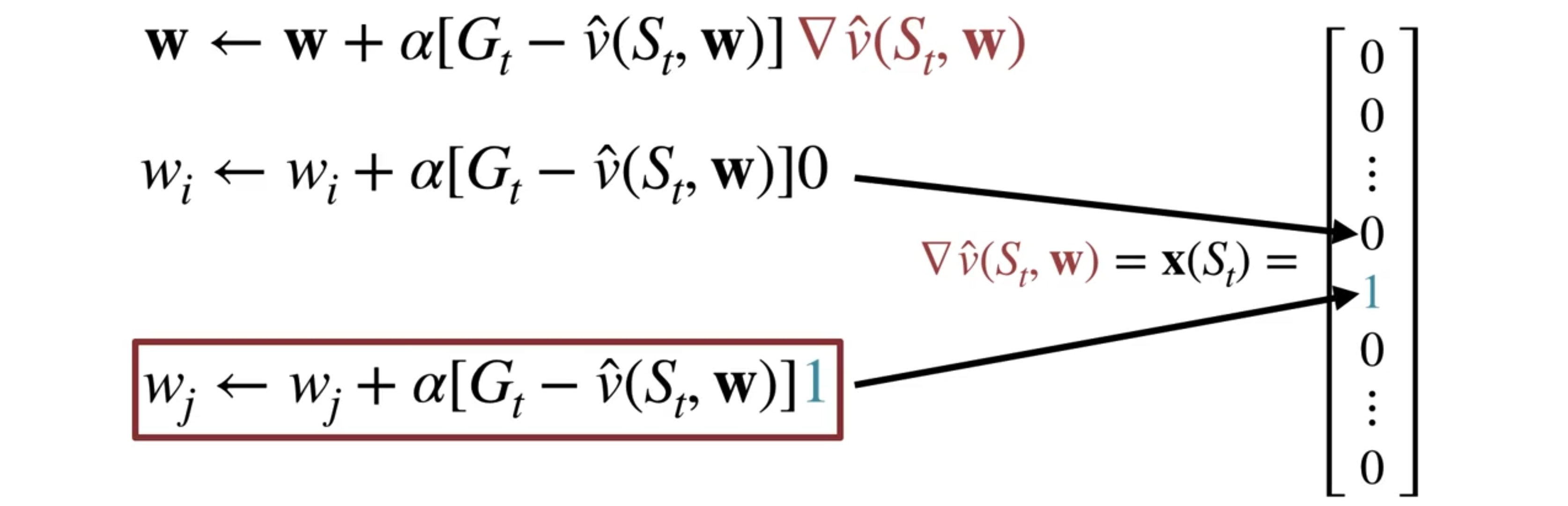
How to Compute the Gradient for MC with State Aggregation

아래 식을 보면 알 수 있듯이,
sample return $v_{\pi}(S_t, w)$보다 $G_t$가 크면 가중치 $w$가 증가한다
반대로의 경우에는 가중치는 감소하고.
그래서 이 문제는 Gradient Descent와 관련있다.

Monte Carlo Updates for a First Episode

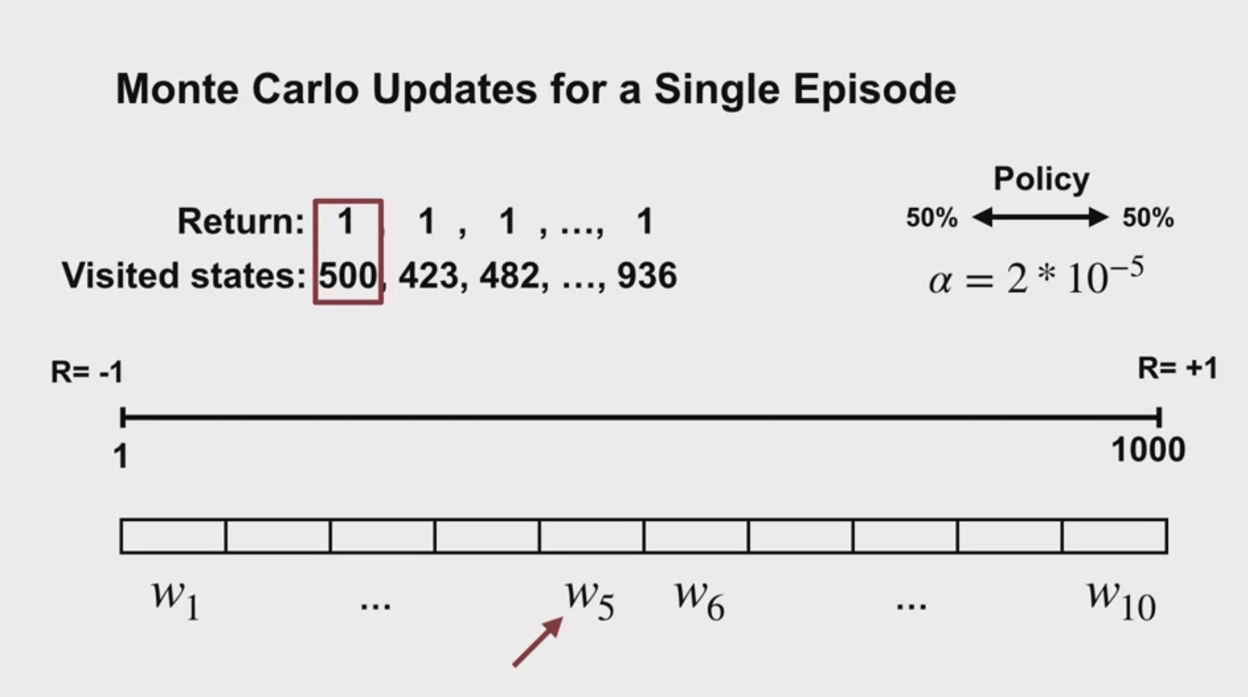
하나의 에피소드, 한 줄의 궤적이 visited states라고 하면
각 위치 숫자는 그 state aggregation 구역에 속하기 때문에
value function이 계단식으로 형성된다.
이 계단의 중심에 true value 직선이 지나간다.

$\mu$는 각 상태에서 얼만큼 시간을 보냈는지에 대한 것임을 고려하면
state aggregation 결과가 계단식으로 출력되는 이유를 이해할 수 있다.

ㄹㄹ