이번엔 피마 인디언 당뇨병 데이터를 이용한 분류 예측을 한다.
지난 학기 데이터마이닝에서 교수님이 활용한 데이터인데, 다시 보니까 반갑다.
데이터 출처: https://www.kaggle.com/datasets/uciml/pima-indians-diabetes-database
피마 인디언 당뇨병 데이터
- Pregnancies: 임신 횟수
- Glucose: 포도당 부하 검사 수치
- BloodPressure: 혈압(mm Hg)
- SkinThickness: 팔 삼두근 뒤쪽의 피하지방 측정값(mm)
- Insulin: 혈청 인슐린(mu U/ml)
- BMI: 체질량지수(체중(kg)/키(m))^2
- DiabetesPedigreeFunction: 당뇨 내력 가중치 값
- Age: 나이
- Outcome: 당뇨병 유무 (0 또는 1)
지금까지 학습한 분류 성능 평가지표들을 이용해보자!
검증 데이터/교차 검증은 하지 않고, 데이터 전처리와 성능 평가지표에 중점을 두자
데이터 확인과 사전 작업
필요한 라이브러리들을 불러오고, 데이터를 확인하자
import numpy as np
import pandas as pd
import matplotlib.pyplot as plt
%matplotlib inline

from sklearn.model_selection import train_test_split
from sklearn.metrics import accuracy_score, precision_score, recall_score, roc_auc_score
from sklearn.metrics import f1_score, confusion_matrix, precision_recall_curve, roc_curve
from sklearn.preprocessing import StandardScaler
from sklearn.linear_model import LogisticRegression

diabetes_data = pd.read_csv('diabetes.csv')
display(diabetes_data.head(3))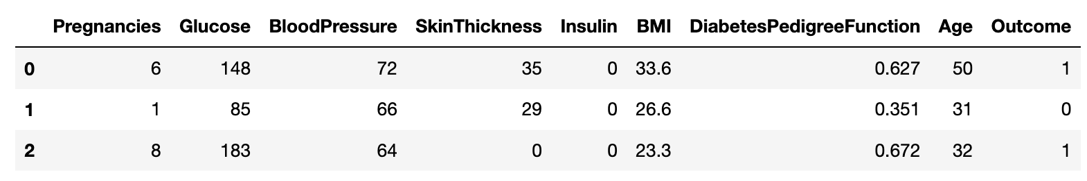
print(diabetes_data['Outcome'].value_counts(), '\n')
print(diabetes_data.info( ))
0 500
1 268
Name: Outcome, dtype: int64
<class 'pandas.core.frame.DataFrame'>
RangeIndex: 768 entries, 0 to 767
Data columns (total 9 columns):
# Column Non-Null Count Dtype
--- ------ -------------- -----
0 Pregnancies 768 non-null int64
1 Glucose 768 non-null int64
2 BloodPressure 768 non-null int64
3 SkinThickness 768 non-null int64
4 Insulin 768 non-null int64
5 BMI 768 non-null float64
6 DiabetesPedigreeFunction 768 non-null float64
7 Age 768 non-null int64
8 Outcome 768 non-null int64
dtypes: float64(2), int64(7)
memory usage: 54.1 KB
None앞에서 만들었던 여러 평가지표를 한번에 출력하는
get_clf_eval()
def get_clf_eval(y_test, pred=None, pred_proba=None):
    confusion = confusion_matrix( y_test, pred)
    accuracy = accuracy_score(y_test , pred)
    precision = precision_score(y_test , pred)
    recall = recall_score(y_test , pred)
    f1 = f1_score(y_test,pred)
    roc_auc = roc_auc_score(y_test, pred_proba)
    print('오차 행렬')
    print(confusion)
    print('정확도: {0:.4f}, 정밀도: {1:.4f}, 재현율: {2:.4f},\
    F1: {3:.4f}, AUC:{4:.4f}'.format(accuracy, precision, recall, f1, roc_auc))
앞에서 만들었던 임곗값에 따른 정밀도와 재현율을 시각화하는
precision_recall_curve_plot()
def precision_recall_curve_plot(y_test=None, pred_proba_c1=None):
    # threshold ndarray와 이 threshold에 따른 정밀도, 재현율 ndarray 추출.
    precisions, recalls, thresholds = precision_recall_curve( y_test, pred_proba_c1)

    # X축을 threshold값으로, Y축은 정밀도, 재현율 값으로 각각 Plot 수행. 정밀도는 점선으로 표시
    plt.figure(figsize=(8,6))
    threshold_boundary = thresholds.shape[0]
    plt.plot(thresholds, precisions[0:threshold_boundary], linestyle='--', label='precision')
    plt.plot(thresholds, recalls[0:threshold_boundary],label='recall')

    # threshold 값 X 축의 Scale을 0.1 단위로 변경
    start, end = plt.xlim()
    plt.xticks(np.round(np.arange(start, end, 0.1),2))

    # x축, y축 label과 legend, 그리고 grid 설정
    plt.xlabel('Threshold value'); plt.ylabel('Precision and Recall value')
    plt.legend(); plt.grid()
    plt.show()
전처리 없이 학습 및 평가
Feature 와 Label로 쪼개고, Train, Test 데이터 분리
(이번에는 Validation 데이터 안 씀)
X = diabetes_data.iloc[:, :-1] # Feature (Outcome 외)
y = diabetes_data.iloc[:, -1] # Label (Outcome)

X_train, X_test, y_train, y_test = train_test_split(X, y, test_size = 0.2, random_state = 156, stratify=y)
LogisticRegression으로 학습 / 예측 후 평가 진행
lr_clf = LogisticRegression(solver='liblinear')
lr_clf.fit(X_train , y_train)
pred = lr_clf.predict(X_test)
pred_proba = lr_clf.predict_proba(X_test)[:, 1]

get_clf_eval(y_test , pred, pred_proba)
오차 행렬
[[87 13]
[22 32]]
정확도: 0.7727, 정밀도: 0.7111, 재현율: 0.5926, F1: 0.6465, AUC:0.8083임곗값에 따른 정밀도와 재현율을 시각화해보자
데이터 전처리 후 더 구체적으로 평가지표를 이용해보자
precision_recall_curve()사용을 위해predict_proba()필요함
pred_proba_c1 = lr_clf.predict_proba(X_test)[:, 1]
precision_recall_curve_plot(y_test, pred_proba_c1)
임곗값 0.47 근처가 괜찮아 보임 (둘 다 적당히 높음)
전처리 후 학습 및 평가
데이터 전처리 후 학습하고, 평가지표들을 좀 더 구체적으로 사용해보자
각 변수들의 기초통계량 확인
display(diabetes_data.describe())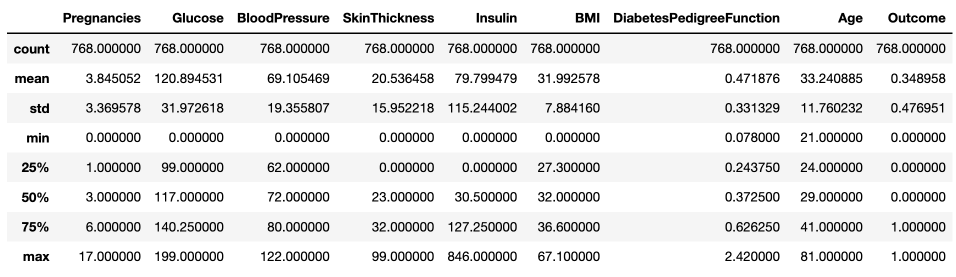
Glucose, BloodPressure, SkinThickness, Insullin, BMI 는 0이 나오면 안 되는 Feature들인데 뭔가 이상하다. 잘못된 값으로 판단하고 정제를 진행하자
Glucose를 히스토그램으로 시각화해보자
plt.hist(diabetes_data['Glucose'], bins=10)
0 값이 떨어져 있음 잘못된 값인 것 같다. 전체 Feature에 대해서 확인해보자
이상하다고 판단되는 변수들에 대해 0 값의 갯수와 비율을 확인하자
# 0값을 검사할 피처명 리스트 객체 설정
zero_features = ['Glucose', 'BloodPressure','SkinThickness','Insulin','BMI']

# 전체 데이터 건수
total_count = diabetes_data['Glucose'].count()

# 피처별로 반복 하면서 데이터 값이 0 인 데이터 건수 추출하고, 퍼센트 계산
for feature in zero_features:
    zero_count = diabetes_data[diabetes_data[feature] == 0][feature].count()
    print('{0} 0 건수는 {1}, 퍼센트는 {2:.2f} %'.format(feature, zero_count, 100*zero_count/total_count))
Glucose 0 건수는 5, 퍼센트는 0.65 %
BloodPressure 0 건수는 35, 퍼센트는 4.56 %
SkinThickness 0 건수는 227, 퍼센트는 29.56 %
Insulin 0 건수는 374, 퍼센트는 48.70 %
BMI 0 건수는 11, 퍼센트는 1.43 %Insulin은 무려 48.7%가 0이었다.
모든 0 값을 각 Feature의 mean 값으로 대체하자
diabetes_data[zero_features]=diabetes_data[zero_features].replace(0, diabetes_data[zero_features].mean())대체가 잘 됐는지 0 값이 갯수와 비율을 다시 한번 보자
# 0값을 검사할 피처명 리스트 객체 설정
zero_features = ['Glucose', 'BloodPressure','SkinThickness','Insulin','BMI']

# 전체 데이터 건수
total_count = diabetes_data['Glucose'].count()

# 피처별로 반복 하면서 데이터 값이 0 인 데이터 건수 추출하고, 퍼센트 계산
for feature in zero_features:
    zero_count = diabetes_data[diabetes_data[feature] == 0][feature].count()
    print('{0} 0 건수는 {1}, 퍼센트는 {2:.2f} %'.format(feature, zero_count, 100*zero_count/total_count))
Glucose 0 건수는 0, 퍼센트는 0.00 %
BloodPressure 0 건수는 0, 퍼센트는 0.00 %
SkinThickness 0 건수는 0, 퍼센트는 0.00 %
Insulin 0 건수는 0, 퍼센트는 0.00 %
BMI 0 건수는 0, 퍼센트는 0.00 %잘 된 것 같다.
Feature와 Label을 나누고, Train, Test 데이터를 나누자
LogisticRegression을 사용할 거니까 Standard 스케일링을 해주자
지금은 연습이니까 그냥 전체 데이터에 대해fit_transfrom()하자
예측 후 평가까지 진행하자
X = diabetes_data.iloc[:, :-1]
y = diabetes_data.iloc[:, -1]

# StandardScaler 클래스를 이용해 피처 데이터 세트에 일괄적으로 스케일링 적용
scaler = StandardScaler( )
X_scaled = scaler.fit_transform(X)

X_train, X_test, y_train, y_test = train_test_split(X_scaled, y, test_size = 0.2, random_state = 156, stratify=y)

# 로지스틱 회귀로 학습, 예측 및 평가 수행.
lr_clf = LogisticRegression()
lr_clf.fit(X_train , y_train)
pred = lr_clf.predict(X_test)
pred_proba = lr_clf.predict_proba(X_test)[:, 1]

get_clf_eval(y_test , pred, pred_proba)
오차 행렬
[[90 10]
[21 33]]
정확도: 0.7987, 정밀도: 0.7674, 재현율: 0.6111, F1: 0.6804, AUC:0.8433여러 전처리를 해주었더니 정밀도와 재현율 모두 상승했다!
이제 이 예측에 대해Binarizer를 이용해서 임곗값을 몇으로 설정하는게 좋을지 확인해보자
실제값, 예측 확률값(predict_proba), 임곗값을 넣으면 임곗값에 따라 평가지표들을 출력하는get_eval_by_threshold()함수를 만들자
from sklearn.preprocessing import Binarizer
def get_eval_by_threshold(y_test , pred_proba_c1, thresholds):
# thresholds 리스트 객체내의 값을 차례로 iteration하면서 Evaluation 수행.
for custom_threshold in thresholds:
binarizer = Binarizer(threshold=custom_threshold).fit(pred_proba_c1)
custom_predict = binarizer.transform(pred_proba_c1)
print('임곗값:',custom_threshold)
get_clf_eval(y_test , custom_predict, pred_proba_c1)
print()임곗값을 리스트로 지정해주고 평가 지표를 확인하자
thresholds = [0.3 , 0.33 ,0.36,0.39, 0.42 , 0.45 ,0.48, 0.50]
pred_proba = lr_clf.predict_proba(X_test)
get_eval_by_threshold(y_test, pred_proba[:,1].reshape(-1,1), thresholds)임곗값: 0.3
오차 행렬
[[67 33]
[11 43]]
정확도: 0.7143, 정밀도: 0.5658, 재현율: 0.7963, F1: 0.6615, AUC:0.8433
임곗값: 0.33
오차 행렬
[[72 28]
[12 42]]
정확도: 0.7403, 정밀도: 0.6000, 재현율: 0.7778, F1: 0.6774, AUC:0.8433
임곗값: 0.36
오차 행렬
[[76 24]
[15 39]]
정확도: 0.7468, 정밀도: 0.6190, 재현율: 0.7222, F1: 0.6667, AUC:0.8433
임곗값: 0.39
오차 행렬
[[78 22]
[16 38]]
정확도: 0.7532, 정밀도: 0.6333, 재현율: 0.7037, F1: 0.6667, AUC:0.8433
임곗값: 0.42
오차 행렬
[[84 16]
[18 36]]
정확도: 0.7792, 정밀도: 0.6923, 재현율: 0.6667, F1: 0.6792, AUC:0.8433
임곗값: 0.45
오차 행렬
[[85 15]
[18 36]]
정확도: 0.7857, 정밀도: 0.7059, 재현율: 0.6667, F1: 0.6857, AUC:0.8433
임곗값: 0.48
오차 행렬
[[88 12]
[19 35]]
정확도: 0.7987, 정밀도: 0.7447, 재현율: 0.6481, F1: 0.6931, AUC:0.8433
임곗값: 0.5
오차 행렬
[[90 10]
 [21 33]]
정확도: 0.7987, 정밀도: 0.7674, 재현율: 0.6111, F1: 0.6804, AUC:0.8433대충 눈으로 봤을 때, 임곗값이 0.48일 때 정밀도와 재현율이 적당히 높아보인다!
최종적으로 임곗값을 0.48로 설정한Binarizer객체를 생성하고
1을 예측하는predict_proba()에 대해fit_transfrom()진행 후 평가해보자
# 임곗값를 0.48로 설정한 Binarizer 생성
binarizer = Binarizer(threshold=0.48)

# 위에서 구한 lr_clf의 predict_proba() 예측 확률 array에서 1에 해당하는 컬럼값을 Binarizer변환.
pred_th_048 = binarizer.fit_transform(pred_proba[:, 1].reshape(-1,1))

get_clf_eval(y_test , pred_th_048, pred_proba[:, 1])
오차 행렬
[[88 12]
[19 35]]
정확도: 0.7987, 정밀도: 0.7447, 재현율: 0.6481, F1: 0.6931, AUC:0.8433