[데이썬☀️_8편] Dacon Basic 실습 설명서(1) - 선형회귀 🐧

거부기·2022년 6월 21일

🌞DACON Day-thon

목록 보기

5/5

데이콘 게시글 중에 서포터즈의 일환으로 직접 쓴 게시글을 정리하기 위해 쓰인 글입니다. PDF 파일의 경우 다음 링크에 들어가시면 다운받을 수 있습니다.
[데이썬☀️_8편] Dacon Basic 실습 설명서(1) - 선형회귀 🐧

안녕하세요! 데이크루 2기 데이썬☀️ 셔휘와 졔이입니다.

드디어 이번 게시글부터는 지금까지 배운 내용을 활용하여 실습에 적용해보는 시간인데요!

실습은 데이콘 Basic에서 🐧펭귄 몸무게 예측 경진대회의 데이터를 활용해 진행해보려고 합니다.
또한 실습에 사용되는 펭귄 데이터는 정형 데이터로 회귀를 활용하여 실습해보도록 하겠습니다.

📣 그럼 이제 데이썬과 함께 펭귄 몸무게 예측 실습을 해보러 가볼까요?

*본 포스팅은 데이콘 서포터즈 “데이크루" 2기 활동의 일환입니다.

✍️ 데이썬의 모든 시리즈 바로가기!

[데이썬☀️_0편] Python으로 시작하는 데이터 분석 사용 설명서

[데이썬☀️_1편] ✏️ 데이터 분석 사용 설명서

[데이썬☀️_2편] 📖 기초 라이브러리 사용 설명서 (1) - Numpy
[데이썬☀️_2편] 📖 기초 라이브러리 사용 설명서 (2) - Pandas
[데이썬☀️_2편] 📖 기초 라이브러리 사용 설명서 (3) - Scikit-learn

[데이썬☀️_3편] 🔍 EDA (탐색적 데이터 분석) 사용 설명서 (1) - EDA & 통계치 분석
[데이썬☀️_3편] 🔍 EDA (탐색적 데이터 분석) 사용 설명서 (2) - Matplotlib
[데이썬☀️_3편] 🔍 EDA (탐색적 데이터 분석) 사용 설명서 (3) - Seaborn
[데이썬☀️_3편] 🔍 EDA (탐색적 데이터 분석) 사용 설명서 (4) - Plotly
[데이썬☀️_3편] 🔍 EDA (탐색적 데이터 분석) 사용 설명서 (5) - Cufflinks

[데이썬☀️_4편] 🛠 전처리 사용 설명서

[데이썬☀️_5편] 🔧 모델링 사용 설명서 (1) - 선형 회귀(Linear Regression)
[데이썬☀️_5편] 🔧 모델링 사용 설명서 (2) - 결정 트리(Decision Tree)
[데이썬☀️_5편] 🔧 모델링 사용 설명서 (3) - 앙상블(Ensemble)

[데이썬☀️_6편] 🤖 모델 검증(validation) 사용 설명서

[데이썬☀️_7편] 🏹 모델 최적화 사용 설명서

🐧 Dacon Basic 실습 설명서(1) - 회귀

데이터 소개
1) 데이터 불러오기
2) 데이터 살펴보기
데이터 탐색(EDA) & 데이터 전처리
1) 결측치 제거하기
2) 데이터 시각화
3) 데이터 인코딩
4) 상관관계 분석
데이터 모델링
1) 릿지 회귀
2) 라쏘 회귀
3) 엘라스틱넷 회귀
예측
1) 결측치 제거하기
2) 인코딩
3) 예측하기

1. 데이터 소개

'펭귄 몸무게 예측 경진대회'는 주어진 펭귄의 종, 부리 길이, 성별 등의 정보들을 이용해 몸무게를 예측하는 대회입니다.

아래 링크에 접속하시면, 데이터를 다운로드 할 수 있습니다. 또한 코드 공유 탭에서 데이콘에서 제공하는 Baseline 코드와 다른 참가자들의 코드도 확인해볼 수 있습니다.😊

🐧 펭귄 몸무게 예측 경진대회

본 게시글은 데이썬의 게시글과 데이콘에서 제공하는 Baseline 코드를 참고하여 작성되었습니다.

📁 펭귄 데이터의 컬럼 정보

id : 일련번호 / 수치형 데이터
Species : 펭귄의 종 / 카테고리형 데이터
Island : 시료를 채취한 섬 / 카테고리형 데이터
Clutch Completion : 연구 둥지가 완전한 클러치(2개의 알)로 관찰되었는지 여부 / 카테고리형 데이터
Culmen Length (mm) : 부리의 등쪽 능선의 길이 (mm) / 수치형 데이터
Culmen Depth (mm) : 부리의 등쪽 능선의 깊이 (mm) / 수치형 데이터
Flipper Length (mm) : 펭귄 지느러미의 길이 (mm) / 수치형 데이터
Sex : 펭귄의 성별 / 카테고리형 데이터
Delta 15 N (o/oo) : 안정 동위원소 15N:14N의 비율 / 수치형 데이터
Delta 13 C (o/oo) : 안정 동위원소 13C:12C의 비율 / 수치형 데이터
Body Mass (g) : 펭귄의 체질량 (g) / 수치형 데이터

출처) https://allisonhorst.github.io/palmerpenguins/reference/penguins_raw.html

1) 데이터 불러오기

먼저 numpy와 pandas를 import하고 학습할 데이터는 train, 예측할 데이터는 test 변수에 저장하겠습니다.

pd.read_csv에 데이터가 저장되어 있는 파일 경로를 지정해주세요!

import numpy as np
import pandas as pd

# 데이터 불러오기
train = pd.read_csv('train.csv')
test = pd.read_csv('test.csv')

2) 데이터 살펴보기

train.head(3)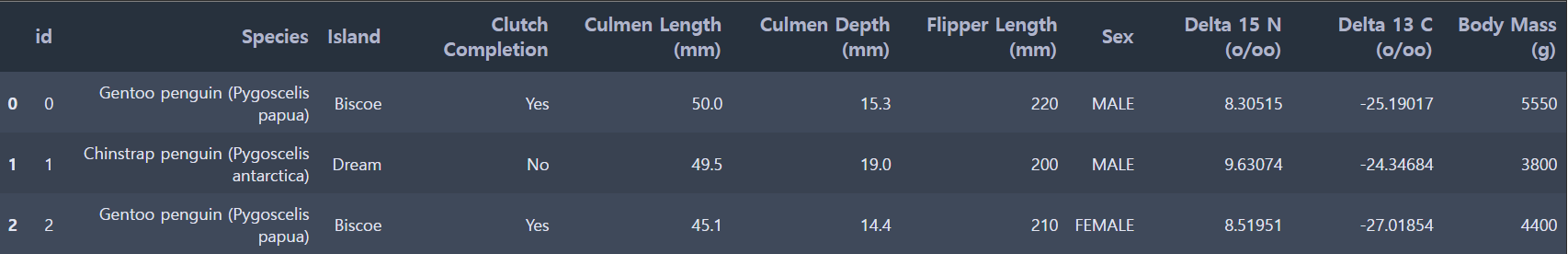

train.info()

<class 'pandas.core.frame.DataFrame'>
RangeIndex: 114 entries, 0 to 113
Data columns (total 11 columns):
 #   Column               Non-Null Count  Dtype  
---  ------               --------------  -----  
 0   id                   114 non-null    int64  
 1   Species              114 non-null    object 
 2   Island               114 non-null    object 
 3   Clutch Completion    114 non-null    object 
 4   Culmen Length (mm)   114 non-null    float64
 5   Culmen Depth (mm)    114 non-null    float64
 6   Flipper Length (mm)  114 non-null    int64  
 7   Sex                  111 non-null    object 
 8   Delta 15 N (o/oo)    111 non-null    float64
 9   Delta 13 C (o/oo)    111 non-null    float64
 10  Body Mass (g)        114 non-null    int64  
dtypes: float64(4), int64(3), object(4)
memory usage: 9.9+ KB

Sex, Delta 15 N (o/oo), Delta 13 C (o/oo) 컬럼에 결측치가 존재합니다.

결측치가 있는 행을 확인해보겠습니다.

train[train.isna().sum(axis=1) > 0]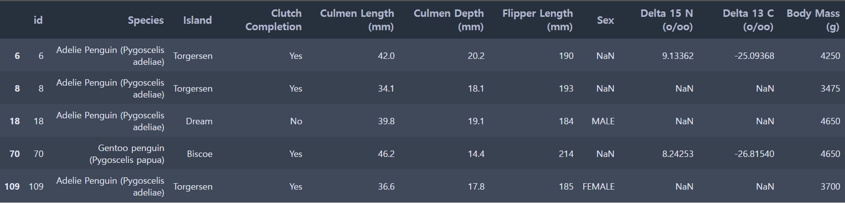

2. 데이터 탐색(EDA) & 데이터 전처리

1) 결측치 제거하기

단순 문자열인 id 컬럼은 예측 성능을 떨어뜨리는 경우가 많기 때문에 삭제해줍니다.

# id 삭제
train = train.drop('id', axis=1)

카테고리형 데이터에 결측치가 존재하는 경우는 행을 삭제하고,

수치형 데이터에 결측치가 존재하는 경우는 0값을 채워주겠습니다.

# 카테고리형 데이터에서 결측치에 해당하는 행 삭제
train_preprocessed = train.dropna(subset=['Sex'])
# 수치형 데이터에서 결측치에 0값 넣기
train_preprocessed = train_preprocessed.fillna(0)
# 확인
train_preprocessed.info()

<class 'pandas.core.frame.DataFrame'>
Int64Index: 111 entries, 0 to 113
Data columns (total 10 columns):
 #   Column               Non-Null Count  Dtype  
---  ------               --------------  -----  
 0   Species              111 non-null    object 
 1   Island               111 non-null    object 
 2   Clutch Completion    111 non-null    object 
 3   Culmen Length (mm)   111 non-null    float64
 4   Culmen Depth (mm)    111 non-null    float64
 5   Flipper Length (mm)  111 non-null    int64  
 6   Sex                  111 non-null    object 
 7   Delta 15 N (o/oo)    111 non-null    float64
 8   Delta 13 C (o/oo)    111 non-null    float64
 9   Body Mass (g)        111 non-null    int64  
dtypes: float64(4), int64(2), object(4)
memory usage: 9.5+ KB

결측치가 모두 제거되었습니다.

2) 데이터 시각화

수치형 데이터와 카테고리형 데이터의 시각화를 따로 진행하기 위해 numeric_feature와 categorical_feature 리스트를 생성해줍니다.

🔢 수치형 데이터
: 'Culmen Length (mm)', 'Culmen Depth (mm)', 'Flipper Length (mm)', 'Delta 15 N (o/oo)', 'Delta 13 C (o/oo)', 'Body Mass (g)'

🔤 카테고리형 데이터
: 'Species', 'Island', 'Clutch Completion', 'Sex'

import matplotlib.pyplot as plt
import seaborn as sns

numeric_feature = ['Culmen Length (mm)', 'Culmen Depth (mm)', 'Flipper Length (mm)', 'Delta 15 N (o/oo)', 'Delta 13 C (o/oo)', 'Body Mass (g)']
categorical_feature = ['Species', 'Island', 'Clutch Completion', 'Sex']

[ 수치형 데이터 시각화 ]

plt.figure(figsize=(15,7))
for i in range(len(numeric_feature)):
  plt.subplot(2,3,i+1)
  sns.boxplot(train[numeric_feature[i]])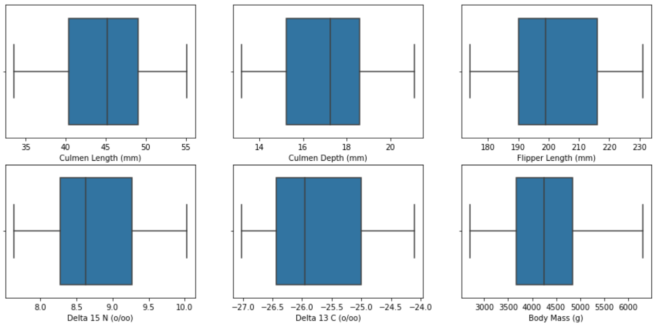

plt.figure(figsize=(15,7)) : figsize=(가로길이,세로길이), 그래프의 크기를 조절
for i in range(len(numeric_feature)) : numeric_feature의 길이만큼 반복문을 수행
plt.subplot(2,3,i+1) : plt.subplot(nrows,ncols,index), 하나의 결과 창에 여러 개의 그래프를 플롯팅할 수 있음 → <2행 3열>
sns.boxplot(train[numeric_feature[i]]) : train 데이터에서 numeric_feature에 해당하는 컬럼의 상자그림을 그림

[ 카테고리형 데이터 시각화 ]

plt.figure(figsize=(12,20))
for i in range(len(categorical_feature)):
  plt.subplot(4,1,i+1)
  sns.barplot(x=categorical_feature[i], y='Body Mass (g)', data=train)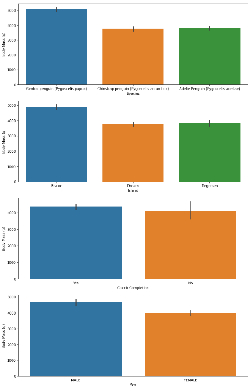

plt.subplot(4,1,i+1) : plt.subplot(nrows,ncols,index), 하나의 결과 창에 여러 개의 그래프를 플롯팅 → <4행 1열>
sns.barplot(x=categorical_feature[i], y='Body Mass (g)', data=train) : train 데이터에서 categorical_feature에 해당하는 컬럼의 막대그래프를 그림, y축 값은 x축 값에 따른 'Body Mass (g)'의 평균

[ 기타 ]
카테고리형 데이터인 'Species', 'Island', 'Sex' 값에 따른 'Body Mass (g)' 값의 차이가 유의미하다고 판단하여

이를 확인해보기 위해 막대그래프와 상자그림을 그려보았습니다.

# Species
plt.figure(figsize=(15,7))

plt.subplot(1,2,1)
plt.xticks(rotation = 90)
sns.barplot(data=train, x='Species', y='Body Mass (g)')
plt.title('The Mean of Body Mess per Species')

plt.subplot(1,2,2)
plt.xticks(rotation = 90)
sns.boxplot(data=train, x='Species',y='Body Mass (g)')
plt.title('Boxplot of Body Mess per Species')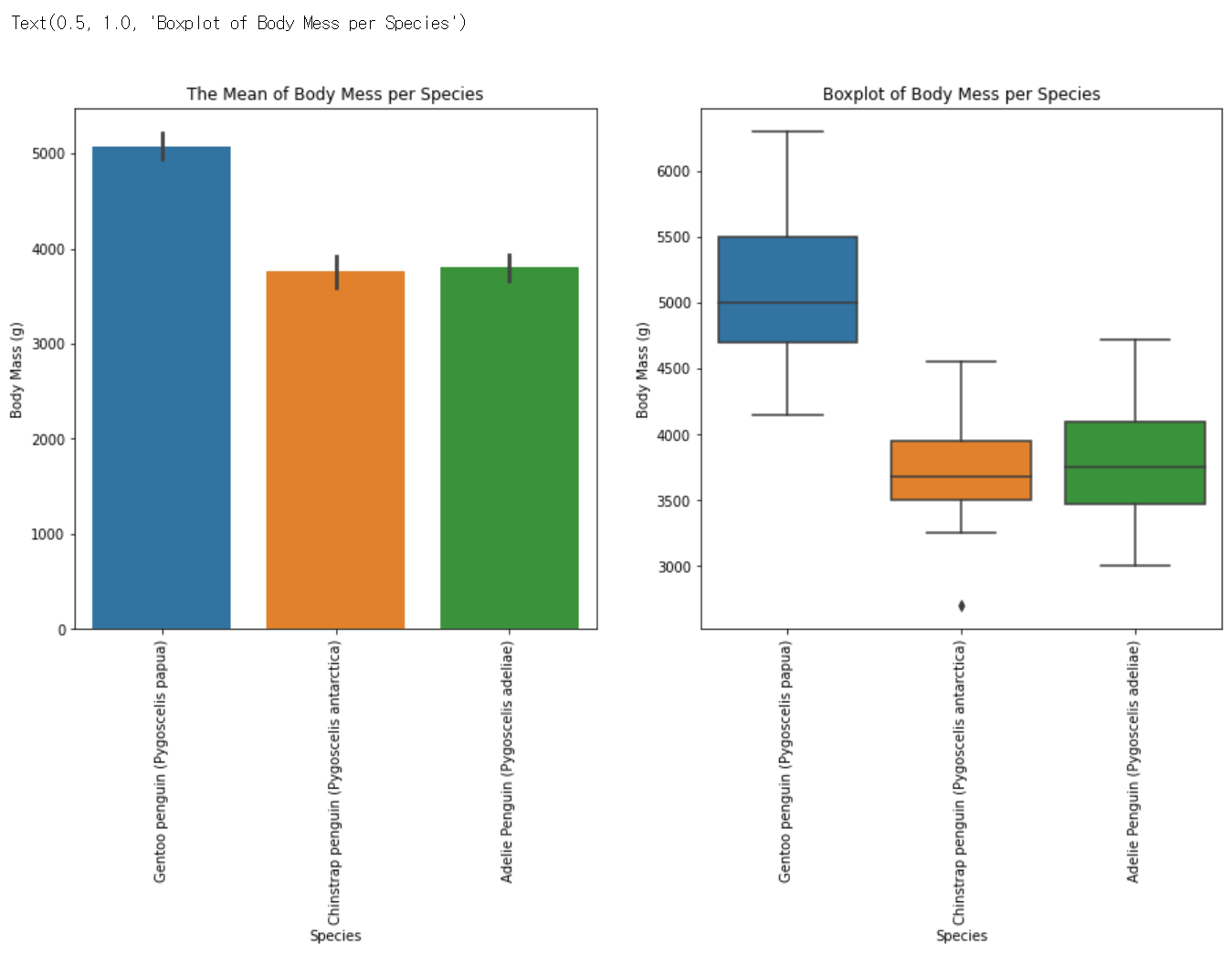

plt.xticks(rotation = 90) : x축 레이블을 회전, x축 레이블의 길이가 길어 겹쳐보이는 문제를 해결하기 위해 90도 회전하였음
sns.barplot(data=train, x='Species', y='Body Mass (g)') : train 데이터에서 'Species'별 'Body Mass (g)'의 막대그래프를 그림, y축 값은 x축 값에 따른 'Body Mass (g)'의 평균
plt.title('The Mean of Body Mess per Species') : 그래프의 제목을 설정
sns.boxplot(data=train, x='Species',y='Body Mass (g)') : train 데이터에서 'Species'별 'Body Mass (g)'의 상자그림을 그림

# Island
plt.figure(figsize=(15,7))

plt.subplot(1,2,1)
sns.barplot(data=train, x='Island', y='Body Mass (g)')
plt.title('The Mean of Body Mess per Island')

plt.subplot(1,2,2)
sns.boxplot(data=train, x='Island',y='Body Mass (g)')
plt.title('Boxplot of Body Mess per Island')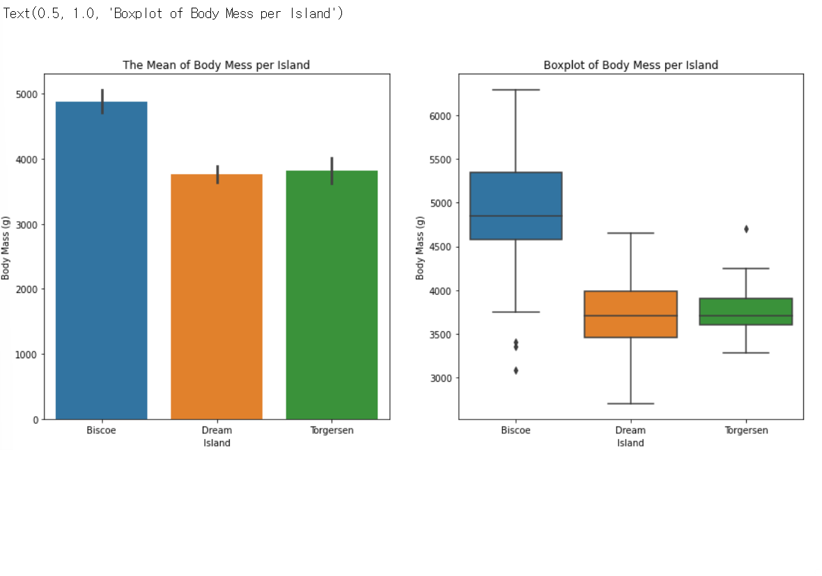

sns.barplot(data=train, x='Island', y='Body Mass (g)') : train 데이터에서 'Island'별 'Body Mass (g)'의 막대그래프를 그림, y축 값은 x축 값에 따른 'Body Mass (g)'의 평균
sns.boxplot(data=train, x='Island',y='Body Mass (g)') : train 데이터에서 'Island'별 'Body Mass (g)'의 상자그림을 그림

# Sex
plt.figure(figsize=(15,7))

plt.subplot(1,2,1)
sns.barplot(data=train, x='Sex', y='Body Mass (g)')
plt.title('The Mean of Body Mess per Sex')

plt.subplot(1,2,2)
sns.boxplot(data=train, x='Sex',y='Body Mass (g)')
plt.title('Boxplot of Body Mess per Sex')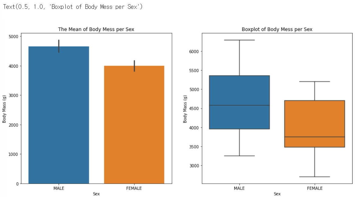

sns.barplot(data=train, x='Sex', y='Body Mass (g)') : train 데이터에서 'Sex'별 'Body Mass (g)'의 막대그래프를 그림, y축 값은 x축 값에 따른 'Body Mass (g)'의 평균
sns.boxplot(data=train, x='Sex',y='Body Mass (g)') : train 데이터에서 'Sex'별 'Body Mass (g)'의 상자그림을 그림

3) 데이터 인코딩

상관관계 분석을 하기에 앞서 상관계수 계산과 모델 학습이 가능하도록 문자열 데이터를 숫자 형으로 바꾸는 과정인 인코딩을 수행하겠습니다.

# 레이블 인코딩을 하기 위한 dictionary map 생성 함수
def make_label_map(dataframe):
    label_maps = {}
    for col in dataframe.columns:
        if dataframe[col].dtype=='object': 
            label_map = {'unknown':0} 
            for i, key in enumerate(train[col].unique()):
                label_map[key] = i+1
            label_maps[col] = label_map
    return label_maps



# 각 범주형 변수에 인코딩 값을 부여하는 함수
def label_encoder(dataframe, label_map):
    for col in dataframe.columns:
        if dataframe[col].dtype=='object':
            dataframe[col] = dataframe[col].map(label_map[col])
            dataframe[col] = dataframe[col].fillna(label_map[col]['unknown']) #혹시 모를 결측값은 unknown의 값으로 채워줍니다.
    return dataframe

# 전처리 완료한 train 데이터 : train_preprocessed
label_map = make_label_map(train_preprocessed) # train_preprocessed 사용해 label map 생성
labeled_train = label_encoder(train_preprocessed, label_map) # train_preprocessed 라벨 인코딩

4) 상관관계 분석

모든 컬럼간의 상관계수를 우선 구한 뒤, seaborn의 heatmap 그래프로 한눈에 보기 쉽게 표현해주도록 하겠습니다.

📊 heatmap이란?
: 데이터를 색상으로 인코딩된 행렬로 표현해주는 그래프로, 값의 차이를 한눈에 파악하기 쉽습니다.

corr = labeled_train.corr()
plt.figure(figsize=(10, 10))
sns.heatmap(corr,
            vmax=0.8,
            linewidths=0.01,
            square=True,
            annot=True,
            cmap='YlGnBu')
plt.title('Feature Correlation')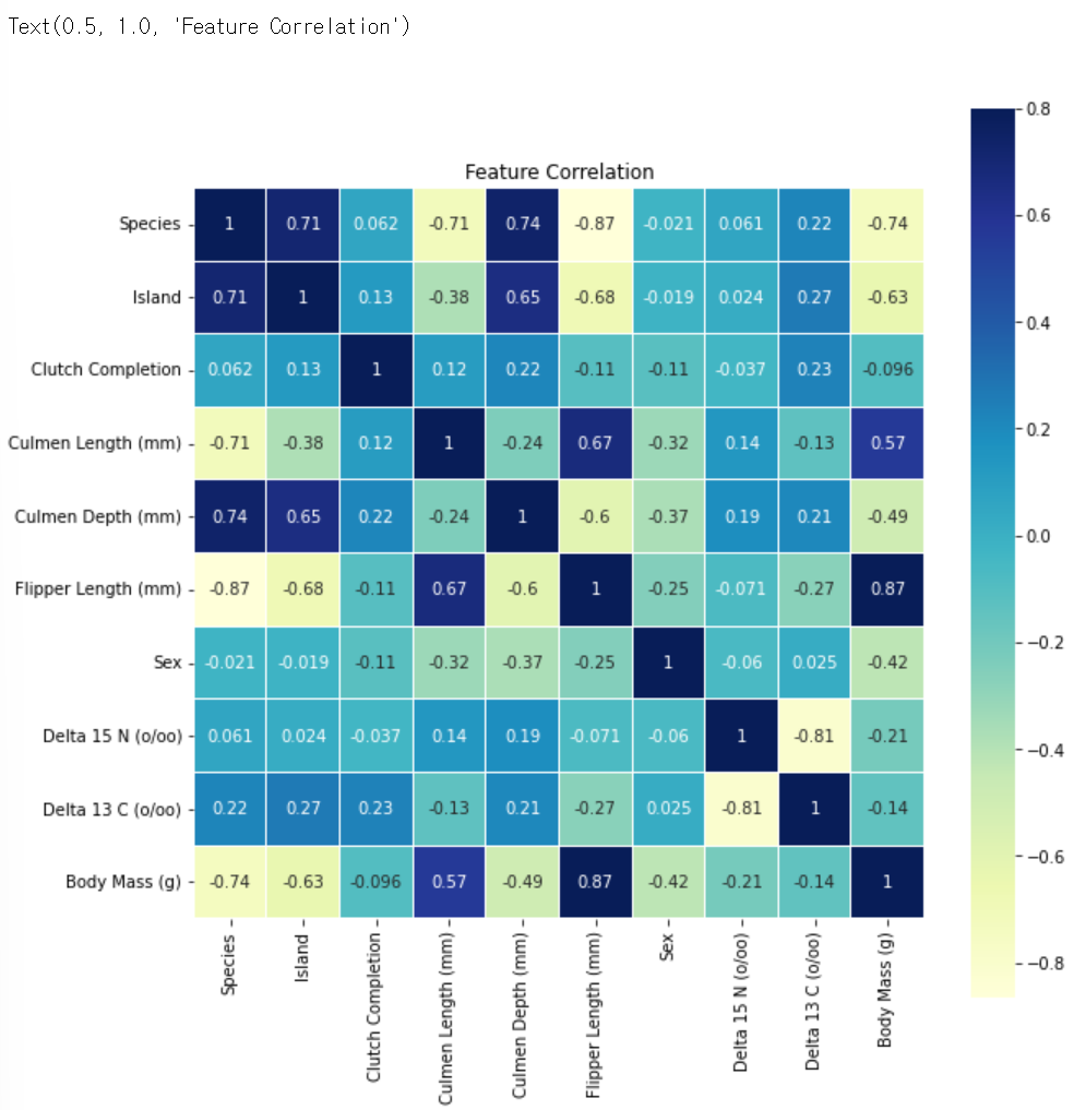

corr = labeled_train.corr() : label_train의 모든 컬럼 간의 상관계수를 구함
sns.heatmap(corr, vmax=0.8, linewidths=0.01, square=True, annot=True, cmap='YlGnBu') : 상관계수 데이터를 heatmap 그래프로 나타냄
▫ vmax : 최댓값
▫ linewidths : 각 셀을 분할할 선의 너비
▫ square : True이면 각 셀이 정사각형 모양이 되도록 설정
▫ annot : True이면 각 셀에 데이터 값을 표시
▫ cmap : 색상 설정

위의 결과 상관계수 값이 0.5를 넘는 수치형 변수의 산점도를 확인해보겠습니다.

Flipper Length (mm) = 0.87 > Species = -0.74 > Island = -0.63 > Culmen Length (mm) = 0.57

plt.figure(figsize=(15,7))

plt.subplot(1,2,1)
sns.scatterplot(data=train, x='Flipper Length (mm)', y='Body Mass (g)')

plt.subplot(1,2,2)
sns.scatterplot(data=train, x='Culmen Length (mm)', y='Body Mass (g)')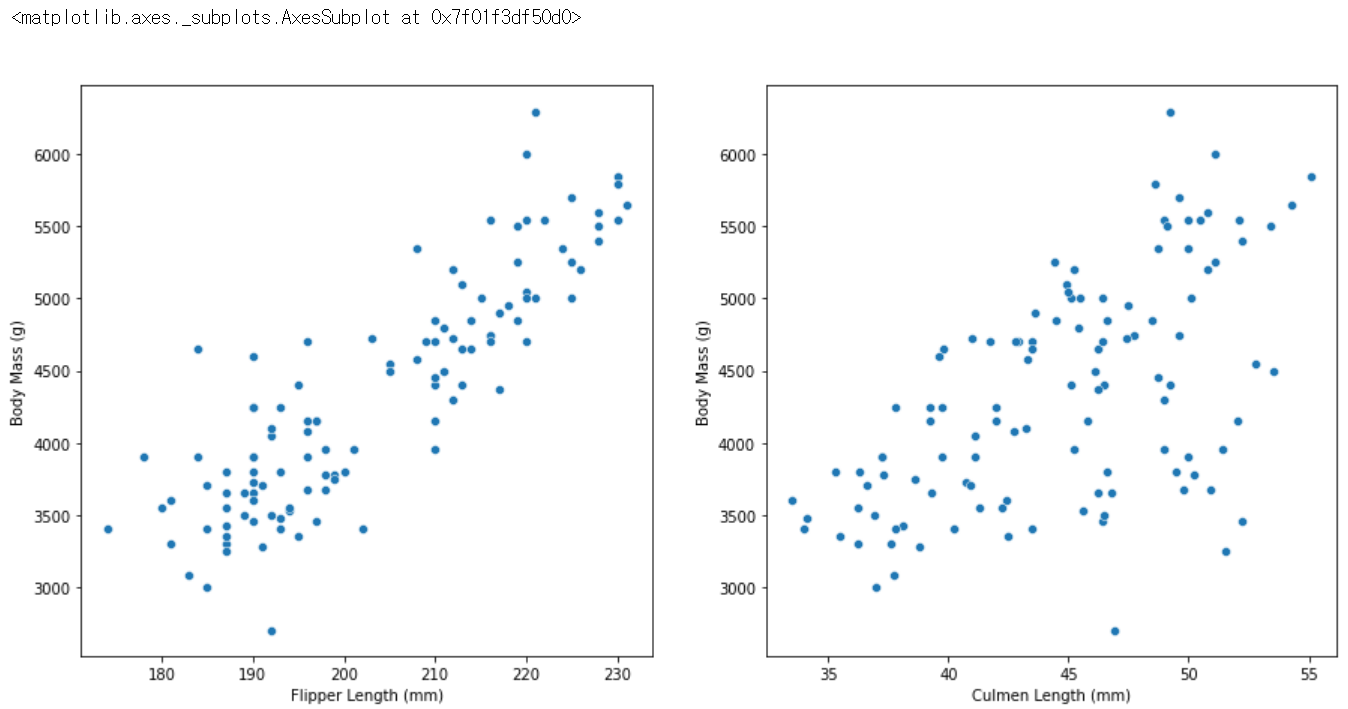

sns.scatterplot(data=train, x='Flipper Length (mm)', y='Body Mass (g)') : 'Flipper Length (mm)'와 'Body Mass (g)'의 산점도를 그림
sns.scatterplot(data=train, x='Culmen Length (mm)', y='Body Mass (g)') : 'Culmen Length (mm)'와 'Body Mass (g)'의 산점도를 그림

seaborn의 regplot 함수는 산점도에 추세선과 95% 신뢰구간이 추가된 그래프입니다.

모든 칼럼과 'Body Mass (g)'칼럼 간의 regplot을 그려 Target과 다른 feature들과의 관계를 살펴보겠습니다.

full_column_list = labeled_train.columns.to_list()
full_column_list.remove('Body Mass (g)')

figure, ax_list = plt.subplots(nrows=3, ncols=3)
figure.set_size_inches(15,15) 

for i in range(len(full_column_list)): 
    sns.regplot(data=labeled_train, x=full_column_list[i], y='Body Mass (g)', 
                ax=ax_list[int(i/3)][int(i%3)], color = "orange")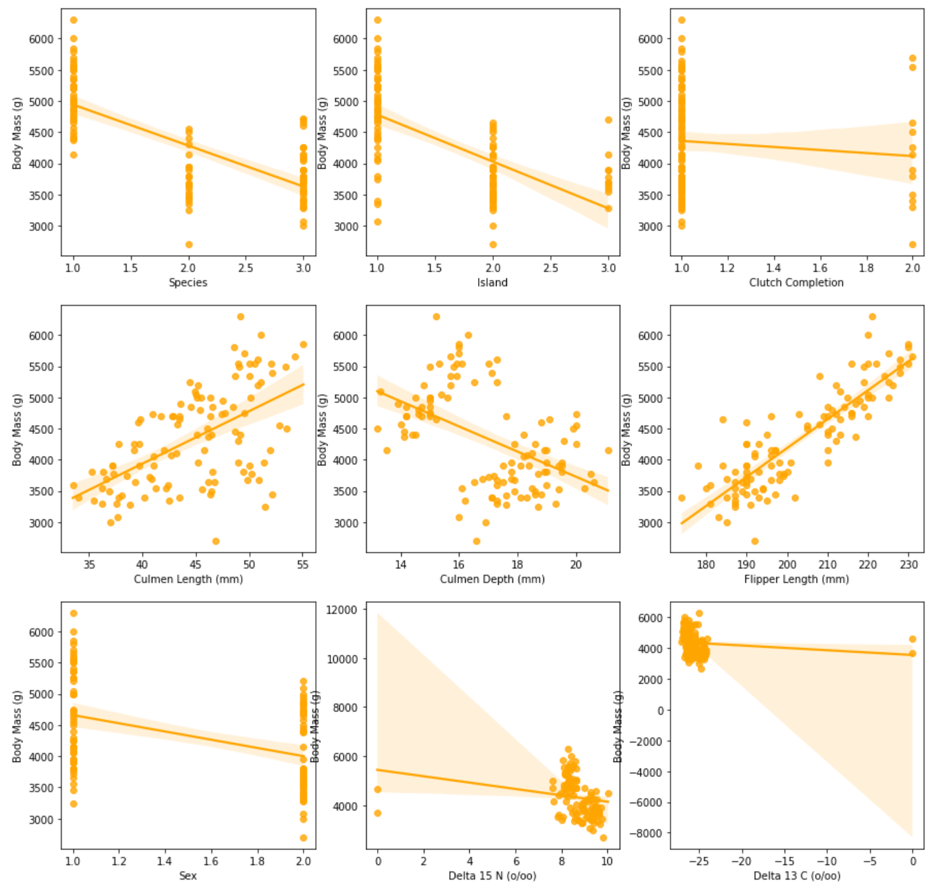

full_column_list

['Species',
 'Island',
 'Clutch Completion',
 'Culmen Length (mm)',
 'Culmen Depth (mm)',
 'Flipper Length (mm)',
 'Sex',
 'Delta 15 N (o/oo)',
 'Delta 13 C (o/oo)']

labeled_train.columns.to_list() : labeld_train의 컬럼 목록을 출력
full_column_list.remove('Body Mass (g)') : Target인 'Body Mass (g)' 칼럼을 제거
figure.set_size_inches(15,15) : 그래프의 크기를 설정
sns.regplot(data=labeled_train, x=full_column_list[i], y='Body Mass (g)', ax=ax_list[int(i/3)][int(i%3)], color = "orange") : 'Body Mass (g)'컬럼과 다른 feature들 간의 regplot을 그림
▫ ax : 플롯을 그릴 축 선택

3. 데이터 모델링

1) 릿지 회귀

릿지(Ridge) 회귀는 W의 제곱에 대해 페널티를 부여하는 L2 규제를 선형 회귀에 적용한 것 입니다.
target과 학습에 불필요한 부분은 제외한 모든 feature은 펭귄몸무게로 지정하고,
alpha 값을 증가시키면 정규화를 통해 회귀 계수가 0에 가까워지므로
Ridge 클래스의 alpha 값을 증가시키면서 회귀를 실행해보겠습니다.

이후 예측 성능을 cross_val_score()로 평가해보겠습니다.

from sklearn.linear_model import Ridge
from sklearn.model_selection import cross_val_score
print('#######  Ridge #######\n')

ridge_alphas = [0, 0.1, 1, 10, 100]

for alpha in ridge_alphas :
    ridge = Ridge(alpha = alpha)

    neg_mse_scores = cross_val_score(ridge, feature, target, scoring="neg_mean_squared_error", cv = 5)
    avg_rmse = np.mean(np.sqrt(-1 * neg_mse_scores))
    print('alpha {0} 일 때 5 folds 의 평균 RMSE : {1:.3f} '.format(alpha, avg_rmse))

#######  Ridge #######

alpha 0 일 때 5 folds 의 평균 RMSE : 336.435 
alpha 0.1 일 때 5 folds 의 평균 RMSE : 336.058 
alpha 1 일 때 5 folds 의 평균 RMSE : 334.030 
alpha 10 일 때 5 folds 의 평균 RMSE : 343.304 
alpha 100 일 때 5 folds 의 평균 RMSE : 380.382

coeff_df = pd.DataFrame()

for pos, alpha in enumerate(ridge_alphas) :
    ridge = Ridge(alpha = alpha)
    ridge.fit(feature, target)
 
    coeff = pd.Series(data=ridge.coef_, index=feature.columns)
    colname = 'alpha:'+str(alpha)
    coeff_df[colname] = coeff

ridge_alphas = [0,  0.1, 1, 10, 100]
sort_column = 'alpha:'+str(ridge_alphas[0])
coeff_df.sort_values(by=sort_column, ascending=False)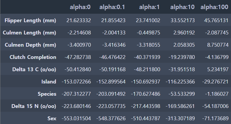

alpha가 1일 때 334.030로 가장 좋은 평균 RMSE를 보여줍니다.

2) 라쏘 회귀

라쏘(Lasso) 회귀는 W의 절댓값에 페널티를 부여하는 L1 규제를 선형 회귀에 적용한 것 입니다.
alpha 값의 변화에 따른 라쏘 회귀 계수 값의 변화를 살펴보겠습니다.

from sklearn.linear_model import Lasso
from sklearn.model_selection import cross_val_score
print('####### Lasso #######\n')

lasso_alphas = [0.07, 0.1, 0.5, 1, 3]

for alpha in lasso_alphas :
    lasso = Lasso(alpha = alpha)

    neg_mse_scores = cross_val_score(lasso, feature, target, scoring="neg_mean_squared_error", cv = 5)
    avg_rmse = np.mean(np.sqrt(-1 * neg_mse_scores))
    print('alpha {0} 일 때 5 folds 의 평균 RMSE : {1:.3f} '.format(alpha, avg_rmse))

####### Lasso #######

alpha 0.07 일 때 5 folds 의 평균 RMSE : 336.335 
alpha 0.1 일 때 5 folds 의 평균 RMSE : 336.292 
alpha 0.5 일 때 5 folds 의 평균 RMSE : 335.737 
alpha 1 일 때 5 folds 의 평균 RMSE : 335.092 
alpha 3 일 때 5 folds 의 평균 RMSE : 332.923

coeff_df = pd.DataFrame()
lasso_alphas = [0.07, 0.1, 0.5, 1, 3]

for pos, alpha in enumerate(lasso_alphas) :
    lasso = Lasso(alpha = alpha)
    lasso.fit(feature, target)
 
    coeff = pd.Series(data=lasso.coef_, index=feature.columns)
    colname = 'alpha:'+str(alpha)
    coeff_df[colname] = coeff

sort_column = 'alpha:'+str(lasso_alphas[0])
coeff_df.sort_values(by=sort_column, ascending=False)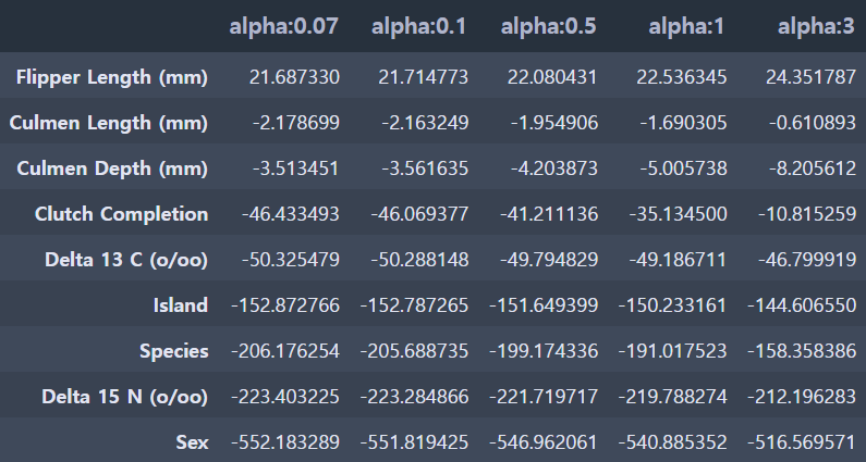

alpha가 3일 때 332.923로 가장 좋은 평균 RMSE를 보여주며, 앞의 릿지 회귀의 평균 RMSE 334.030보다 더 좋은 수치입니다.

3) 엘라스틱넷 회귀

이번엔 L2 규제와 L1 규제를 결합한 엘라스틱넷(Elastic Net) 회귀를 해보겠습니다.
다시 alpha 값의 변화에 따른 엘라스틱넷 회귀 계수 값의 변화를 살펴보겠습니다.

from sklearn.linear_model import ElasticNet
from sklearn.model_selection import cross_val_score

print('####### ElasticNet #######')

elastic_alphas = [0.07, 0.1, 0.5, 1, 3]

for alpha in elastic_alphas :
    elastic = ElasticNet(alpha = alpha, l1_ratio=0.7)

    neg_mse_scores = cross_val_score(elastic, feature, target, scoring="neg_mean_squared_error", cv = 5)
    avg_rmse = np.mean(np.sqrt(-1 * neg_mse_scores))
    print('alpha {0} 일 때 5 folds 의 평균 RMSE : {1:.3f} '.format(alpha, avg_rmse))

####### ElasticNet #######
alpha 0.07 일 때 5 folds 의 평균 RMSE : 333.500 
alpha 0.1 일 때 5 folds 의 평균 RMSE : 333.745 
alpha 0.5 일 때 5 folds 의 평균 RMSE : 347.653 
alpha 1 일 때 5 folds 의 평균 RMSE : 360.314 
alpha 3 일 때 5 folds 의 평균 RMSE : 377.953

coeff_df = pd.DataFrame()
elastic_alphas = [0.07, 0.1, 0.5, 1, 3]

for pos, alpha in enumerate(elastic_alphas) :
    elastic = ElasticNet(alpha = alpha, l1_ratio=0.7)
    elastic.fit(feature, target)
 
    coeff = pd.Series(data=elastic.coef_, index=feature.columns)
    colname = 'alpha:'+str(alpha)
    coeff_df[colname] = coeff

sort_column = 'alpha:'+str(elastic_alphas[0])
coeff_df.sort_values(by=sort_column, ascending=False)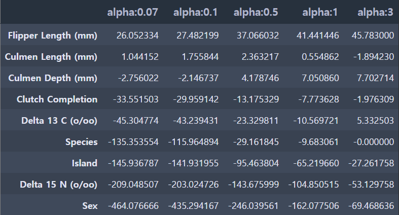

alpha가 0.07일 때 333.500로 가장 좋은 평균 RMSE를 보여주며,
라쏘 회귀보다는 아니지만 릿지 회귀의 평균 RMSE 343.304보다는 더 좋은 수치입니다.

회귀분석 결과

👉 릿지 회귀, 라쏘 회귀, 엘라스틱넷 회귀 결과 라쏘 회귀의 RMSE 결과가 가장 적게 나왔습니다.
RMSE가 낮을 수록 회귀 성능이 좋은 것이기 때문에, 펭귄 몸무게 예측에는 라쏘 회귀가 가장 적절한 모델임을 알 수 있습니다.

4. 예측

1) 결측치 제거하기

test 데이터를 가져와 데이터를 확인합니다.
또한 .info()를 통해 결측치가 있는지 살펴봅니다.

test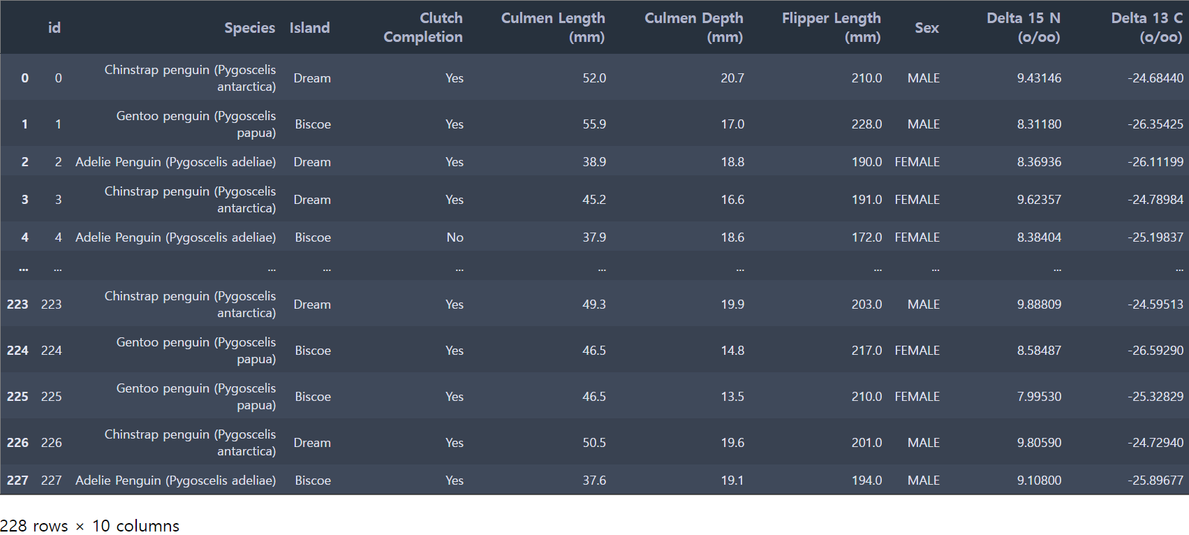

test.info()

<class 'pandas.core.frame.DataFrame'>
RangeIndex: 228 entries, 0 to 227
Data columns (total 10 columns):
 #   Column               Non-Null Count  Dtype  
---  ------               --------------  -----  
 0   id                   228 non-null    int64  
 1   Species              228 non-null    object 
 2   Island               228 non-null    object 
 3   Clutch Completion    228 non-null    object 
 4   Culmen Length (mm)   228 non-null    float64
 5   Culmen Depth (mm)    228 non-null    float64
 6   Flipper Length (mm)  228 non-null    float64
 7   Sex                  222 non-null    object 
 8   Delta 15 N (o/oo)    219 non-null    float64
 9   Delta 13 C (o/oo)    220 non-null    float64
dtypes: float64(5), int64(1), object(4)
memory usage: 17.9+ KB

test 데이터에서 Sex, Delta 15 N (o/oo),Delta 13 C (o/oo) 이렇게 총 3개의 컬럼에서 결측치가 존재함을 알 수 있습니다.

이전에 공부했던 것을 떠올리면 결측치를 채울 수 있는 다양한 방법들이 있었는데요,
저희 데이썬은 카테고리형 데이터인 Sex 컬럼의 결측치는 해당하는 행의 최빈값으로 대체해보겠습니다.

test['Sex']
test['Sex'].value_counts()

MALE      112
FEMALE    110
Name: Sex, dtype: int64

test_preprocessed = test

test_preprocessed['Sex'] = test['Sex'].fillna("MALE")
test_preprocessed['Sex'].value_counts()

MALE      118
FEMALE    110
Name: Sex, dtype: int64

다시 test 데이터를 살펴보며, Sex 컬럼의 결측치가 제거됐는지 확인하고, 나머지 결측치가 있는 컬럼의 결측치를 제거하는 작업을 진행합니다

test_preprocessed.info()

<class 'pandas.core.frame.DataFrame'>
RangeIndex: 228 entries, 0 to 227
Data columns (total 10 columns):
 #   Column               Non-Null Count  Dtype  
---  ------               --------------  -----  
 0   id                   228 non-null    int64  
 1   Species              228 non-null    object 
 2   Island               228 non-null    object 
 3   Clutch Completion    228 non-null    object 
 4   Culmen Length (mm)   228 non-null    float64
 5   Culmen Depth (mm)    228 non-null    float64
 6   Flipper Length (mm)  228 non-null    float64
 7   Sex                  228 non-null    object 
 8   Delta 15 N (o/oo)    219 non-null    float64
 9   Delta 13 C (o/oo)    220 non-null    float64
dtypes: float64(5), int64(1), object(4)
memory usage: 17.9+ KB

test_preprocessed['Delta 15 N (o/oo)']

0      9.43146
1      8.31180
2      8.36936
3      9.62357
4      8.38404
        ...   
223    9.88809
224    8.58487
225    7.99530
226    9.80590
227    9.10800
Name: Delta 15 N (o/oo), Length: 228, dtype: float64

test_preprocessed['Delta 15 N (o/oo)'].describe()

count    219.000000
mean       8.731226
std        0.544827
min        7.685280
25%        8.325385
50%        8.675380
75%        9.109330
max       10.023720
Name: Delta 15 N (o/oo), dtype: float64

test_preprocessed['Delta 15 N (o/oo)'] = test_preprocessed['Delta 15 N (o/oo)'].fillna(0)
test_preprocessed['Delta 13 C (o/oo)'] = test_preprocessed['Delta 13 C (o/oo)'].fillna(0)

수치형인 데이터인 결측치가 존재했던 Delta 15 N (o/oo)과 Delta 13 C (o/oo) 컬럼에 결측값으로 0을 채워줍니다.

이후 id 컬럼을 삭제한 후, 결측치가 있는 컬럼이 더 이상 없는지와 id 컬럼이 삭제 됐는지 확인합니다.
아래 결과를 보면 결측치가 존재하지 않고 id 컬럼이 삭제된 것을 볼 수 있습니다.

test_preprocessed= test_preprocessed.drop('id', axis=1)
test_preprocessed.info()

<class 'pandas.core.frame.DataFrame'>
RangeIndex: 228 entries, 0 to 227
Data columns (total 9 columns):
 #   Column               Non-Null Count  Dtype  
---  ------               --------------  -----  
 0   Species              228 non-null    object 
 1   Island               228 non-null    object 
 2   Clutch Completion    228 non-null    object 
 3   Culmen Length (mm)   228 non-null    float64
 4   Culmen Depth (mm)    228 non-null    float64
 5   Flipper Length (mm)  228 non-null    float64
 6   Sex                  228 non-null    object 
 7   Delta 15 N (o/oo)    228 non-null    float64
 8   Delta 13 C (o/oo)    228 non-null    float64
dtypes: float64(5), object(4)
memory usage: 16.2+ KB

2) 인코딩

결측치를 처리한 test 데이터에 범주형 변수들이 문자열의 형태로 존재하고 있습니다.
모델학습이 가능하도록 문자열 형태의 범주형 변수를 숫자 형태로 인코딩해주는 라벨 인코딩을 진행해줍니다.

def make_label_map(dataframe):
    label_maps = {}
    for col in dataframe.columns:
        if dataframe[col].dtype=='object': 
            label_map = {'unknown':0} 
            for i, key in enumerate(train[col].unique()):
                label_map[key] = i+1
            label_maps[col] = label_map
    return label_maps


# 전처리 완료한 test 데이터 : test_preprocessed
label_map = make_label_map(test_preprocessed) 
labeled_test = label_encoder(test_preprocessed, label_map)

labeled_test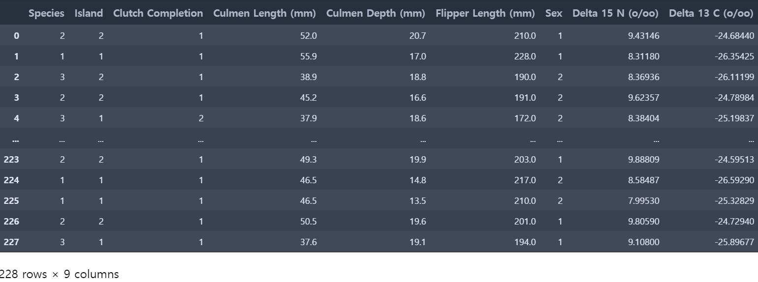

3) 예측하기

앞서 회귀분석 결과에서 라쏘 회귀가 적절한 모델이였기 때문에, predict을 사용하여 예측을 진행합니다.
이후 예측된 결과값을 DataFrame 형식으로 생성한 후 cvs 파일로 저장해주며, 실습이 마무리 됩니다.

new_x_pred = lasso.predict(labeled_test)

ans = pd.DataFrame(new_x_pred)
ans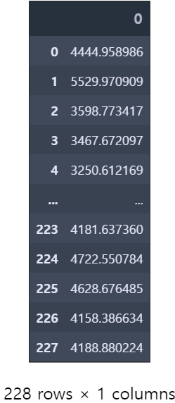

ans.to_csv('ans.csv')

이렇게 펭귄 몸무게 예측 데이터를 활용하여 회귀 실습을 진행해 보았습니다.

배운 내용을 실습에 젹용해보고, 더 다양한 방법을 적용해볼 수 있는 실습이라 더 재미있었는데요!
여러분들도 글을 보시고 여러분의 방법으로 실습을 진행해보셨길 바랍니다🦾

다음엔 데이썬의 마지막이자 두번째 실습 게시글이 업로드될 예정입니다!
손동작 데이터에 앙상블을 활용한 실습이니 많이 기대해주세요🤓

그럼 마지막까지 많은 관심과 애정 부탁드려요! 감사합니다💛

거부기

느리지만 확실하게

이전 포스트

[데이썬☀️_8편] Dacon Basic 실습 설명서(1) - 선형회귀 🐧

🌞DACON Day-thon

✍️ 데이썬의 모든 시리즈 바로가기!

🐧 Dacon Basic 실습 설명서(1) - 회귀

1. 데이터 소개

1) 데이터 불러오기

2) 데이터 살펴보기

2. 데이터 탐색(EDA) & 데이터 전처리

1) 결측치 제거하기

2) 데이터 시각화

3) 데이터 인코딩

4) 상관관계 분석

3. 데이터 모델링

1) 릿지 회귀

2) 라쏘 회귀

3) 엘라스틱넷 회귀

회귀분석 결과

4. 예측

1) 결측치 제거하기

2) 인코딩

3) 예측하기

[데이썬☀️_6편] 🤖 모델 검증(validation) 사용 설명서

0개의 댓글