✨ Accelerated MRI에 필요한 Dataset에 관한 논문
(읽기 전 주의!) Fourier Transform 등 수학적으로 자세한 설명 or 정리는 담지 않았다.
- MRI의 가속화(accelerate) -> acquisition time에 따른 환자의 stress, 비용, artifact 감소
목적: scan time을 줄여도 AI를 통해 기존의 긴 scan time만큼 좋은 이미지를 얻는 것
🍞 1. Introduction
MRI Imaging Speed를 높이기 위한 여러 노력들에 대해 소개한다.
Parallel Imaging, Compressed Sensing(CS), Machine Learning(ML) 등등...
하지만 large-scale의 public dataset은 FastMRI 이전까지 없었다. 😥
--> 8344 volumes, 167,375 slices를 포함한 large-scale dataset인 FastMRI 두둥등장
🍞 2. Introduction to MR Image Acquisition and Reconstruction
MR Imaging은 Frequency와 Phase를 통해 이미지를 얻는 indirect한 과정이다.
공간적, 일시적으로 바뀌는 자기장 "pulse sequence"를 통해 환자 몸의 전자기 공명 -> receiver coil로 측정
---> 다차원 공간인 k-space 데이터 획득
MR Imaging은 이 k-space 데이터를 Inverse Fourier Transform(IFT)을 통해 얻는다!
2.1 Parallel MR Imaging
- 여러 receiver coil을 사용하여 각각 서로 다른 k-space matrix 생성
- accelerated MR에서는 k-space signal이 undersampling
section 2.2, 3은 생략!
🍞 4. The fastMRI Dataset and Associated Tasks
http://fastmri.med.nyu.edu/ -> 이쪽에서 간단한 정보 작성 후 데이터를 받을 수 있다.
knee / brain MR 데이터고,
-
Raw multi-coil k-space data: 복소수 값을 가지는 multi-coil MR 측정 data
-
Emulated single-coil k-space data: multi-coil을 single coil로 합쳐놓은 것 (비교적 multi-coil보다 간단)
-
Ground-truth images: 실수 값의 fully-sampled 된 multi-coil MR 측정 data
- root-sum-of-squares 된 reconstruction reference -
DICOM images: raw data가 제거된 spatially-resolved image
Train, val, test, challenge subset들을 제공하며, test와 challenge에는 GT X
4.1 ~ 4.9 Anonymization ~ Cartesian Undersampling
익명화부터 무릎은 1.5T, 뇌는 1.5T/3T, T1 T2 FLAIR 다 있고... undersampling은 어떻게 했고 등등
데이터셋과 연관된 태스크에 관한 정보들을 적어놓은 섹션이다.
🍞 5. Metrics
MRI reconstruction quality에 대한 평가를 어떻게 할 것인가?
- Normalized Mean Squared Error
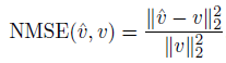
선명도(sharpness)보다는 부드러움(smoothness)을 선호하는 경향이 있기 때문에, 다른 지표들도 사용 권장.
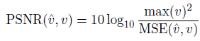
- Peak Signal-to-Noise Ratio(PSNR)
- Structural Similarity
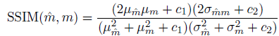
SSIM을 계산할 때는 평균, 분산, 공분산과 같은 통계적 측정치를 기반으로, 두 이미지 간의 밝기(luminance), 대비(contrast), 구조(structure)의 유사성을 평가한다.
값은 -1~1의 범위고, 1은 두 이미지가 완벽하게 일치함을 나타낸다.
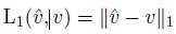
- L1 Loss
🍞 6. Baseline Models
다양한 크기의 train data subset에서 다양한 크기의 여러 U-Net 모델을 train
-> 더 큰 양의 데이터로 train 시 reconstruction quality ↑
🍞 7. Discussion - 8. Conclusion
아무튼 이 대규모 FastMRI 데이터셋을 통해 MR reconstruction의 발전을 기대한다 ~~
👀 간단한 실습 코드
FastMRI 깃허브에서 제공하는 FastMRI tutorial을 바탕으로 실습해보자!
# 필요 라이브러리 로드
import h5py
import numpy as np
from matplotlib import pyplot as plt

file_name = 'h5 파일 경로'
hf = h5py.File(file_name)

print('Keys:', list(hf.keys()))
print('Attrs:', dict(hf.attrs))
로드된 파일의 keys를 출력하면, k-space와 reconstruction_rss를 각각 확인할 수 있다.
volume_kspace = hf['kspace'][()]
print(volume_kspace.dtype)	# complex64
print(volume_kspace.shape)	# (35,15,640,368)
# 15 = coil 개수, 640x368 = img size
slice_kspace = volume_kspace[20] # Choosing the 20-th slice of this volume
def show_coils(data, slice_nums, cmap=None):
fig = plt.figure()
for i, num in enumerate(slice_nums):
plt.subplot(1, len(slice_nums), i + 1)
plt.imshow(data[num], cmap=cmap)
show_coils(np.log(np.abs(slice_kspace) + 1e-9), [0, 5]) # This shows coils 0, 5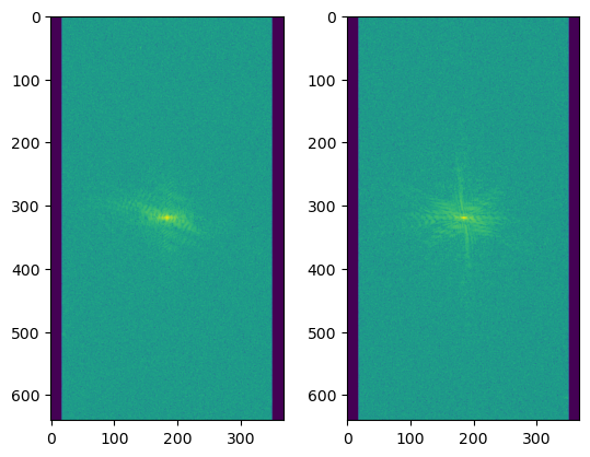
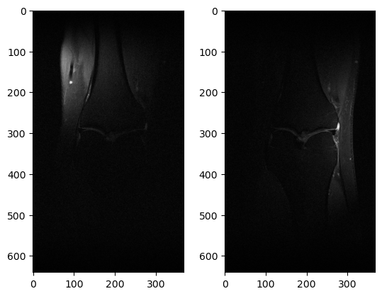
# use fastmri
import fastmri
from fastmri.data import transforms as T

slice_kspace2 = T.to_tensor(slice_kspace)      # Convert from numpy array to pytorch tensor
slice_image = fastmri.ifft2c(slice_kspace2)           # Apply Inverse Fourier Transform to get the complex image
slice_image_abs = fastmri.complex_abs(slice_image)   # Compute absolute value to get a real image

show_coils(slice_image_abs, [0, 5], cmap='gray')
slice_image_rss = fastmri.rss(slice_image_abs, dim=0)
plt.imshow(slice_image_rss.numpy(), cmap='gray')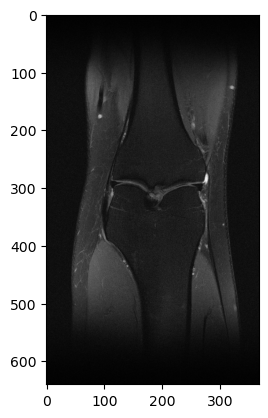
이제 fully-sampled는 다 봤으니까, undersampling 해보자!
from fastmri.data.subsample import RandomMaskFunc, EquiSpacedMaskFunc
#mask_func = RandomMaskFunc(center_fractions=[0.04], accelerations=[8])  # Create the mask function object
mask_func = EquiSpacedMaskFunc(center_fractions=[0.08], accelerations=[4])

# 실제로는 random보다 equispacemaskfunc을 더 많이 쓴당
# 8배 가속화는 cf = 0.04(4%), 4배 가속화는 cf=0.08(8%)

volume_tensor = T.to_tensor(volume_kspace)
masked_kspace, mask, _ = T.apply_mask(volume_tensor, mask_func)   # Apply the mask to k-space
print(masked_kspace.shape) # torch.Size([35, 15, 640, 368, 2]) -> 2는 real / complex
sampled_image = fastmri.ifft2c(masked_kspace)           # Apply Inverse Fourier Transform to get the complex image
sampled_image_abs = fastmri.complex_abs(sampled_image)   # Compute absolute value to get a real image
sampled_image_rss = fastmri.rss(sampled_image_abs, dim=1)	# coil의 dim은 1번째니까 dim=1로 rss 해주는거임

plt.imshow(np.abs(sampled_image_rss[20].numpy()), cmap='gray')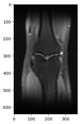
이렇게 가속화된 이미지를 input/reconstruction_rss를 label로 설정하여 recon 모델을 짜볼 수 있다.