3D Gaussian Splatting 완벽 분석 (feat. CUDA Rasterizer)

Hwan Heo·2024년 7월 31일

3D GS 3D Gaussian Splatting Neural Rendering rasterization

Neural Rendering

목록 보기

15/16

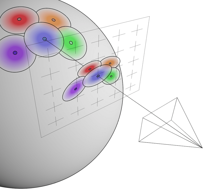
figure credit: Luma AI

들어가며

3D Gaussian Splatting 의 최대 장점은 그 무엇보다도 100fps 이상의 렌더링 '속도' 이다.
그 어떤 NeRF-based method 보다도 빠른 이 속도는 잘 설계된 tile-based rasterization 덕분인데, 오늘은 이 rasterization 관점에서 3D Gaussin Splatting 을 (최대한) 완벽하게 이해해보는 시간을 갖도록 해보자.

1. 3D Gaussian as Primitive Kernel

3D Gaussian Splatting 의 기본 idea 는, implicit 한 NeRF 와 다르게 explicit 하고 학습 가능한 primitives 로 scene 을 표현하자는 것이다. (explicit 한 표현으로 갖는 여러가지 장점이 있는데, 이는 저번 2D GS review 에서 언급한 바 있으니 궁금하다면 링크를 참조하기 바란다.)

저자들은 이러한 primitive (particle) 에 대한 kernel 을 다음과 같은 3D Gaussian function 으로 정의하였다.

G(x) = \exp \left( {- \frac{1}{2} x^{\rm T} \Sigma^{-1} x} \right )

이 kernel design 에 대해서 꼭 3D Gaussian 이어야 했나? 라는 의문이 들 수 있는데, 논문에 언급된 몇 가지 도입 이유가 있다.

학습을 위해 differentiable 할 것
빠른 alpha blending 을 위해서 2D 로의 projection 이 쉽고 잘 정의되어 있을 것

해당 기준 정도만 만족하면 어떤 kernel design 을 사용해도 무방할 것 같고, 실제로 최근 3D Gaussian Ray Tracing 에서 여러가지 kernel 로 실험해봤는데, 성능에 큰 차이 없었다고 한다.

Covariance Matrix 는 positive definite 일 때만 물리적인 의미를 가지므로, 저자들은 학습의 용이성을 위해 covariance matrix 를 다음과 같은 형태로 구성할 것을 제안한다. ( $R,\ S \ \in \mathbb{R}^{3 \times 3}$ rotation, scale matrix)

\Sigma = RSS^{\rm T}R^{\rm T}

이 covariance matrix 를 다음과 같이 약간 바꿔서 쓸 수 있는데,

\begin{aligned} \Sigma & = R (SS^{\rm T}) R^{\rm T} \\ & = R \begin{bmatrix} s_1^2 & 0 & 0 \\ 0 & s_2^2 & 0 \\ 0 & 0 & s_3^2 \\ \end{bmatrix} R^{\rm T} \end{aligned}

covariance matrix 의 형태가 3D ellipsoid (anistropic) matrix 와 같은 것을 알 수 있다. 즉 3D GS 는 3D 상의 불투명한 (Gaussian Distribution 으로 density 가 정의되는) 타원체를 primitive kernel 로 사용한 것이다.

Tip. Quadratic form ( $A^{-1}MA$ ) 을 다룰 때는, $M$ transformation in $A$ coordinate system 이라고 해석하면 좋을 때가 많다.
$\ {}$ 이는 eigendecomposition 을 해석할 때도 마찬가지인데, 선형변환에도 방향이 보존되는 axis (eigenvectors) 로 이루어진 coordinate system 에서, 각 axis 가 어느 정도의 가중치를 가지고 있는지 (eigenvalues) 분석하는 것이 eigendecomposition 이다. 이렇게 생각하면 PCA 가 왜 eigendecomposition 과 연관있는지 자명하다.

다시 말해, 정의된 Covariance matrix 는

ellipsoid 의 각 principal axis 가 basis 인 coordinate system 에서의 intensity matrix (squared scale) 를
world coordinate system 으로의 표현 방법

이라고도 해석할 수 있다.

<Corresponding CUDA Code>

glm::mat3 S = glm::mat3(1.0f);
S[0][0] = mod * scale.x;
S[1][1] = mod * scale.y;
S[2][2] = mod * scale.z;

glm::mat3 R = glm::mat3(
	1.f - 2.f * (y * y + z * z), 2.f * (x * y - r * z), 2.f * (x * z + r * y),
	2.f * (x * y + r * z), 1.f - 2.f * (x * x + z * z), 2.f * (y * z - r * x),
	2.f * (x * z - r * y), 2.f * (y * z + r * x), 1.f - 2.f * (x * x + y * y)
);

glm::mat3 M = S * R;
glm::mat3 Sigma = glm::transpose(M) * M;

cov3D[0] = Sigma[0][0];
cov3D[1] = Sigma[0][1];
cov3D[2] = Sigma[0][2];
cov3D[3] = Sigma[1][1];
cov3D[4] = Sigma[1][2];
cov3D[5] = Sigma[2][2];

여기서

S: 3x3 diagonal matrix,
R: quaternion to rotation matrix 공식을 통해서 계산되었다. $R = \begin{bmatrix} 1 - 2y^2 - 2z^2 & 2xy - 2zw & 2xz + 2yw \\ 2xy + 2zw & 1 - 2x^2 - 2z^2 & 2yz - 2xw \\ 2xz - 2yw & 2yz + 2xw & 1 - 2x^2 - 2y^2 \end{bmatrix}$
COV: symmetric 이므로, right upper triangle 만 저장해도 된다.

임을 유의하자.

2. Splatting (Projection of Primitives)

2.1. Projection

이제 world system 위에 정의된 gaussian 의 covariance matrix 를 image space 에 projection 할 방법이 필요한데, 저자들은 EWA Splatting 에서 제안된, 다음과 같은 방법으로 이를 해결한다.

\Sigma^{\prime} = JW\Sigma (JW)^{\rm T}

이 식의 의미를 조금 더 자세히 분석해보도록 하자.

이 변환에도 quadratic form 에 대해 같은 해석이 가능하다: 즉, world coordinate system → camera space → ray space 에서의 covariance matrix 를 의미한다.
여기서 $J$ 는, Jacobian (affine approximation) of the perspective projection (camera space to ray space), 다시 말해 camera → ray space transformation $\phi$ 에 대한 linear approximation 이다.

\phi(x) = \phi(t) + J \cdot (x - t)

1st order Taylor approximation 이기 때문에, Gaussian 중심에서 멀어질수록 approximation error 가 생길 것임이 자명하다. 최근에는 이러한 perspective error 를 3D GS 의 한계로 제시하고 해결하려는 연구들도 제시되고 있다. (2D Gaussian Splatting / On the error analysis of 3D Gaussian Splatting)

Perspective projection 에 대한 Jacobian $J$ 는 다음과 같이 유도되며,

\begin{bmatrix} 1 / t_2 & 0 & -t_0 / t_2^2 \\ 0 & 1 / t_2 & -t_1 / t_2^2 \\ t_0 / \| t\| & t_1 / \| t\| & t_2 / \| t\| \\ \end{bmatrix}

실제 구현에서는

image space pixel $(u,v)$ 가 pinhole camera model 에서 다음과 같고

$(u,v) = ( \frac{xf}{z}, \frac{yf}{z})$
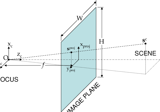
image space 에서 필요한 covariance matrix 는 2x2 형태이기 때문에 projection 된 covariance 의 3rd row (z-axis) 는 실제로 사용되지 않으므로

아래의 형태로 구현되어 있다.

\begin{bmatrix} f_x / t_2 & 0 & -f_x \cdot t_0 / t_2^2 \\ 0 & f_y / t_2 & - f_y \cdot t_1 / t_2^2 \\ 0 & 0 & 0 \\ \end{bmatrix}

<Corresponding CUDA Code>

// Affine approximation of the Jacobian matrix of viewmatrix to rayspace
glm::mat3 J = glm::mat3(
	focal_x / t.z, 0.0f, -(focal_x * t.x) / (t.z * t.z),
	0.0f, focal_y / t.z, -(focal_y * t.y) / (t.z * t.z),
	0, 0, 0);

// W: w2c matrix 
glm::mat3 W = glm::mat3(
	viewmatrix[0], viewmatrix[4], viewmatrix[8],
	viewmatrix[1], viewmatrix[5], viewmatrix[9],
	viewmatrix[2], viewmatrix[6], viewmatrix[10]);
    
glm::mat3 T = W * J;
glm::mat3 Vrk = glm::mat3(
	cov3D[0], cov3D[1], cov3D[2],
	cov3D[1], cov3D[3], cov3D[4],
	cov3D[2], cov3D[4], cov3D[5]);

glm::mat3 cov = glm::transpose(T) * glm::transpose(Vrk) * T;

COV3D 를 symmetricity 이용해서 upper right triangle 만 저장했으므로 그 점 고려해서 load 하는 것을 유의하자.

2.2. Density of the Projected Gaussian

실제 rendering 시에는 Gaussian density 값과 opacity 값을 곱하여 사용하기 때문에, 3D 공간 위의 점 $p$ 에 대해, $i$ th Gaussian 의 density $f_i(p)$ 를 다음과 같이 정의할 수 있다.

f_i(p) = \sigma(\alpha_i) \exp \left( - \frac{1}{2} (\mu_i -p)^{\rm T} \Sigma_i^{-1} (\mu_i - p ) \right )

이는 multivariate (3D) normal distribution 에 대한 weighted (opacity) probability density function 라고도 볼 수 있다.
inner exponential 의 값은 Mahalanobis Distance 인데, 3D 상에서 이 값은 scale 을 고려한 ellipsoid 내에서 거리 ( Similarity) 라고 볼 수 있다. 즉, 어떤 3D 상의 point 에서, Gaussian 과 가까울수록, Gaussian 이 opaque 할수록 response 가 커야하는 직관과 정확히 일치한다.

위 density 값을 계산하려면 projection 된 covaraiance 의 inverse matrix 가 필요하다. 코드 상으론 inverse 를 구하는 과정에서 선형대수를 이용한 트릭이 좀 있으니 살펴보도록 하자.

앞서 계산한 2D covariance matrix 를 구하는 함수 끝이 실제로는 다음과 같으며,

cov[0][0] += 0.3f;
cov[1][1] += 0.3f;

return { float(cov[0][0]), float(cov[0][1]), float(cov[1][1]) };

이는

A^{\rm T}A+\lambda \mathbf{I}

의 inverse matrix 를 구하는 것과 동일한 것을 알 수 있다. $(A=RS)$

covariance matrix 가 positive semidefinite 이기 때문에, small $\lambda$ 를 더해주면 다음과 같이 covariance matrix 가 positive definite 이 되므로,

x^T A^T Ax + \lambda x^T x > 0

이 트릭을 통해 inverse matrix 를 구할 때 numerical unstability 가 방지된다.

float det = (cov.x * cov.z - cov.y * cov.y);
if (det == 0.0f)
	return;
float det_inv = 1.f / det;
float3 conic = { cov.z * det_inv, -cov.y * det_inv, cov.x * det_inv };

Recap. 2x2 matrix 의 inverse matirx formula 는 다음과 같음을 기억하자

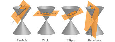
A=\begin{bmatrix} a & b \\ b & c \end{bmatrix}, \quad A^{-1} = \frac{1}{\det(A)} \begin{bmatrix} c & -b \\ -b & a \end{bmatrix}

또한 cov 의 inverse 를 conic 이라고 명명하고 있는데, 이는 아마 ellipsoid 등이 conic section 으로 정의되기 때문인 것 같다.

마지막으로 각 splats 의 radius 를, 99.7% 이상 cover 가능한

r = 3 \times \max_i \textit{standard deviation}_i

으로 정의해서, 이 값을 Gaussian culling (masking) 하는 용도로 사용한다. (그렇지 않으면 scene 안의 모든 Gaussian 에 query 해야 한다….)

Covariance matrix 로 정의된 3D Gaussian 의 standard deviation 은 eigenvalue 와 같으므로, 다음의 Characteristic equation

\det \left ( A -\lambda \mathbf{I} \right ) = 0, \\ \rightarrow (a- \lambda)(c-\lambda) - b^2 = 0

을 푸는 것으로 standard deviation 을 구할 수 있다.

이는 $\lambda$ 에 대한 2차 방정식이므로, 너무나 유명한 closed form solution (근의 공식) 이 존재한다 :) 코드에도 근의 공식을 통해 lambda 값을 구하도록 되어있다.

float mid = 0.5f * (cov.x + cov.z);
float lambda1 = mid + sqrt(max(0.1f, mid * mid - det));
float lambda2 = mid - sqrt(max(0.1f, mid * mid - det));

float my_radius = ceil(3.f * sqrt(max(lambda1, lambda2)));

3. Rasterization

Gaussian kernel 의 정의와, 이 kernel 이 image space 상에 어떻게 projection 되는지 알고 있으므로, 이제 우리는

ray 와 intersect 하는 Gaussian 들에 대해
density 와 opacity 값을 depth order 로만 정렬해서 모으면

3D GS scene 을 2D image 로 그릴 수 있다.

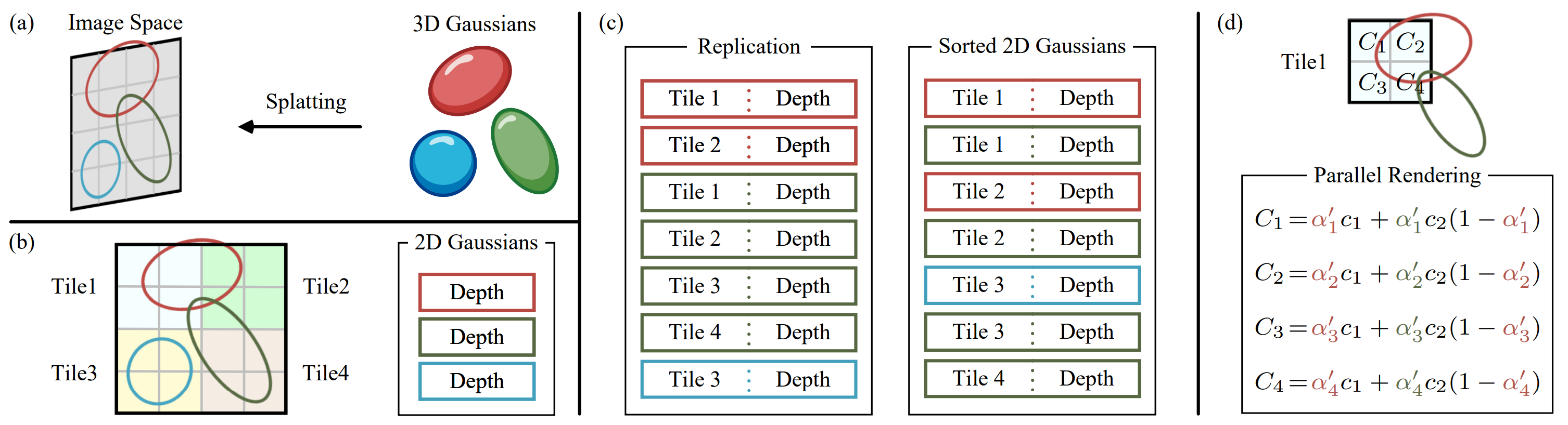
3D Gaussian Splatting 은 이러한 rendering 작업을 효율적으로 하기 위하여 image space (screen) 에 모든 3D Gaussian 을 projection 한 후, 작은 단위의 tile 로 나누어서 각 tile 마다 color / opacity accumulation 을 병렬로 실행하는 tile-based rasterization 을 제시하였다.

논문에 제시된 Rasterization algorithm 을 step-by-step 으로 분석해보도록 하자.

Screen 을 16x16 크기의 tile 로 나눈다.
- 이는 CUDA 병렬화 작업을 위해 <<< 전체 tile 개수, 256 >>> 의 grid, thread block 으로 나누어 rasterization 을 진행하기 위함이다.
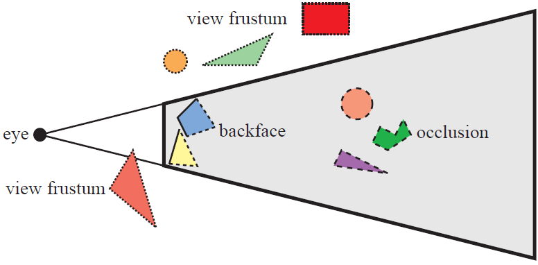
Frustum culling 으로 valid gaussian 만 남긴다. (See fig.)
Tile 마다 겹치는 Gaussian 은 복제하여 사용한다. (Instantiate)
(각 tile 에서) Gaussian 을 depth order 로 정렬한다 (using GPU radix sort)
- Rendering 할 때 사용하는 covariance 가 이미 image space 에 projection 된 상태이므로, depth 로 sort 하지 않으면 순서 없이 이리저리 겹쳐져 있는 모습과 같을 것이다.
- 이 sorting 은 각 thread block 실행 전에 진행되어 tile 단위로는 sort 를 진행하지 않는다. 즉 pre-sort primitives!
정렬된 Gaussian 를 통해 각 tile 마다 작업 범위를 설정하고, Tile 마다 one CUDA thread block 을 실행하여 병렬로 rasterize 를 진행한다.
- 각 thread block 은 메모리 병목을 줄이기위해 몇 가지 정보를 shared memory 에 저장해놓는다.
- 정렬된 Gaussian 을 따라서 opacity, color 를 accumulate 하여 최종 color 값을 계산한다.

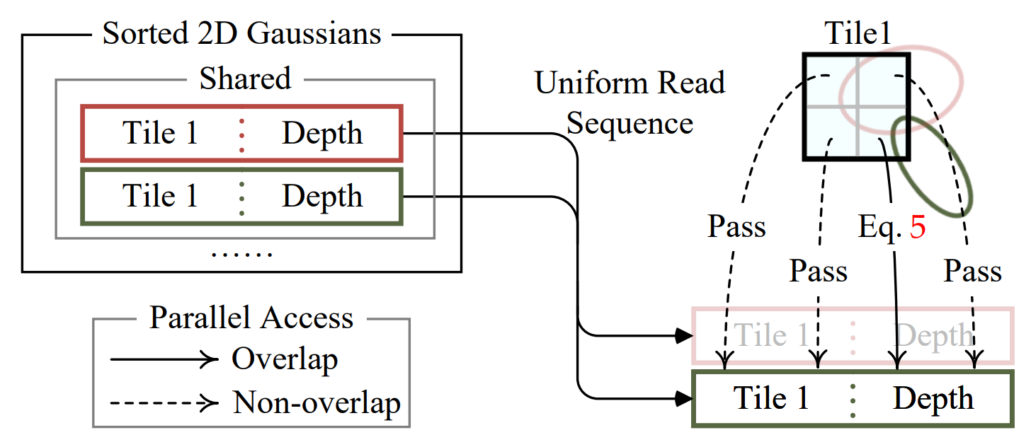
shared variable 에 실제로 id, opacity, pixel coord 등의 값을 저장해놓고 있도록 구현되어 있다. 즉 Gaussian 의 projected covariance, spherical harmoics color 등은 tile 단위의 계산이 일어나기 전에 이미 계산을 마치고 shared memory 에 저장되어 있다.

// Allocate storage for batches of collectively fetched data.
__shared__ int collected_id[BLOCK_SIZE];
__shared__ float2 collected_xy[BLOCK_SIZE];
__shared__ float4 collected_conic_opacity[BLOCK_SIZE];

또한 (5) 의 color 계산을 위한 accumulation 과정을 공식으로 써보면 다음과 같은데,

C(\mathbf{x}) = \sum_{i \in N} T_i \, g_i^{2D}(x) \, \alpha_i \, \mathbf{c}_i , \quad \text{where } T_i = \prod_{j=1}^{i-1} \left(1 - g_j^{2D}(x) \, \alpha_j\right)

여기서도 NeRF 와의 차이점을 볼 수 있다.

Ray 를 따라 point 를 sampling 하여 그 point 의 opacity / color 를 MLP 에 query 해야하는 NeRF 와 달리,
3D GS 에서는 이미 tile 에 projection 된 $N$ 개의 splats 를 depth order 로 탐색하면서 opacity / color 를 합한다.
즉 NeRF 에서는 ray 를 sampling 하기 때문에 $r(t)$ 로 sampling 된 각각 다른 point 를 MLP 에 query 하지만, 3D GS 는 모두 똑같은 점 $x$ 를 query 하는 것을 볼 수 있다.

// Iterate over the current batch
for (int j = 0; !done && j < min(BLOCK_SIZE, toDo); j++)
{
	// xy: the 2d coord of the Gaussian center
	// pixf: the 2d coord of the current pixel
	// con_o: inv cov2d (x,y,z), opacity (w)
    float2 xy = collected_xy[j];
	float2 d = { xy.x - pixf.x, xy.y - pixf.y };
	float4 con_o = collected_conic_opacity[j];
	
	// density = -1/2 * (d^T inv(cov2d) d)
	float density = -0.5f * (con_o.x * d.x * d.x + con_o.z * d.y * d.y) - con_o.y * d.x * d.y;
	if (density > 0.0f)
		continue;

	// response = density * opacity
	float alpha = min(0.99f, con_o.w * exp(density));
	if (alpha < 1.0f / 255.0f)
		continue;

	// alpha blending, from near to far
	float test_T = T * (1 - alpha);
	if (test_T < 0.0001f)
	{
		done = true;
		continue;
	}

	// Eq. (3) from 3D Gaussian splatting paper.
	for (int ch = 0; ch < CHANNELS; ch++)
		C[ch] += features[collected_id[j] * CHANNELS + ch] * alpha * T;

	T = test_T;
}

4. 그 외 이모저모

4.1. Camera Model

현재 구현상으로는 $J$ 가 pinhole camera model 의 perspective projection 으로 구현되었기 때문에 다른 camera model 로 rendering 이 불가능하지만, $J$ matrix 를 알맞은 camera model 에 대해 modeling 하면 원하는 camera model 에 대한 rendering 이 가능하다.

일례로, spherical camera model (e.g., equirectangular) 에 대한 matrix $J$ 를 다음과 같이 modeling 할 수 있는데,

	float t_length = sqrtf(t.x * t.x + t.y * t.y + t.z * t.z);

	float3 t_unit_focal = {0.0f, 0.0f, t_length};
	glm::mat3 J = glm::mat3(
		focal_x / t_unit_focal.z, 0.0f, -(focal_x * t_unit_focal.x) / (t_unit_focal.z * t_unit_focal.z),
		0.0f, focal_x / t_unit_focal.z, -(focal_x * t_unit_focal.y) / (t_unit_focal.z * t_unit_focal.z),
		0, 0, 0);

이를 통해 다음의 360 image 를 3D GS 를 통해 training / rendering 이 가능하다.

Original	GS ptc

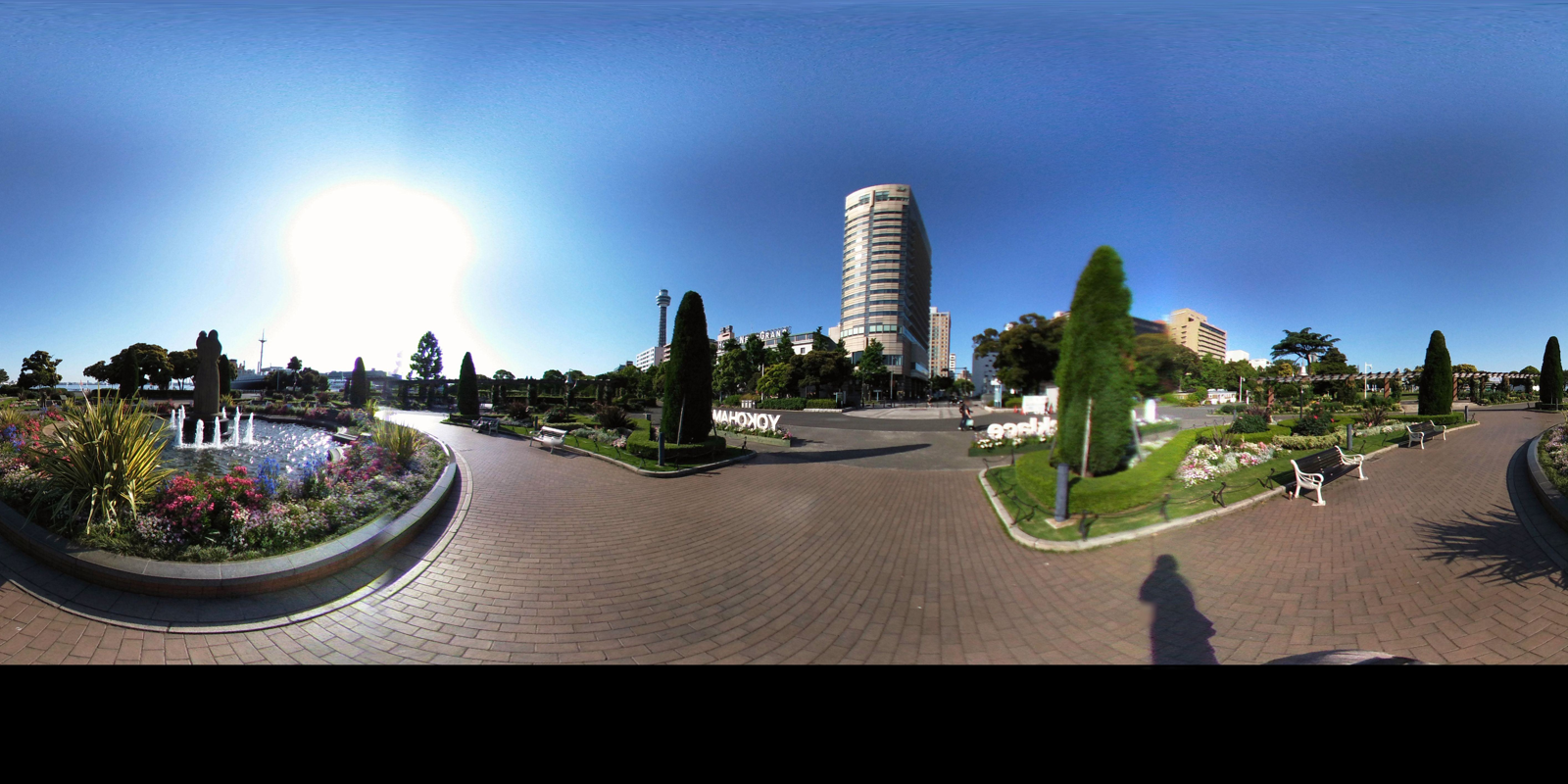물론 이 경우에는 approximation error 가 perspective projection 보다 훨씬 커지게되어 PNSR 이 pinhole images 를 사용할 때보다 낮아지게 된다. affine projection 을 사용하지 않고 rendering 을 구현하여 camera modeling 하는 방법도 있지만 이는 추후 소개하도록 하겠다.

4.2. Mimic Luma AI

글 Teaser 의 동영상은 NeRFStudio 팀이 창업한 Luma AI 의 rendering 영상인데, 꽤나 팬시해서 따라해보았다.

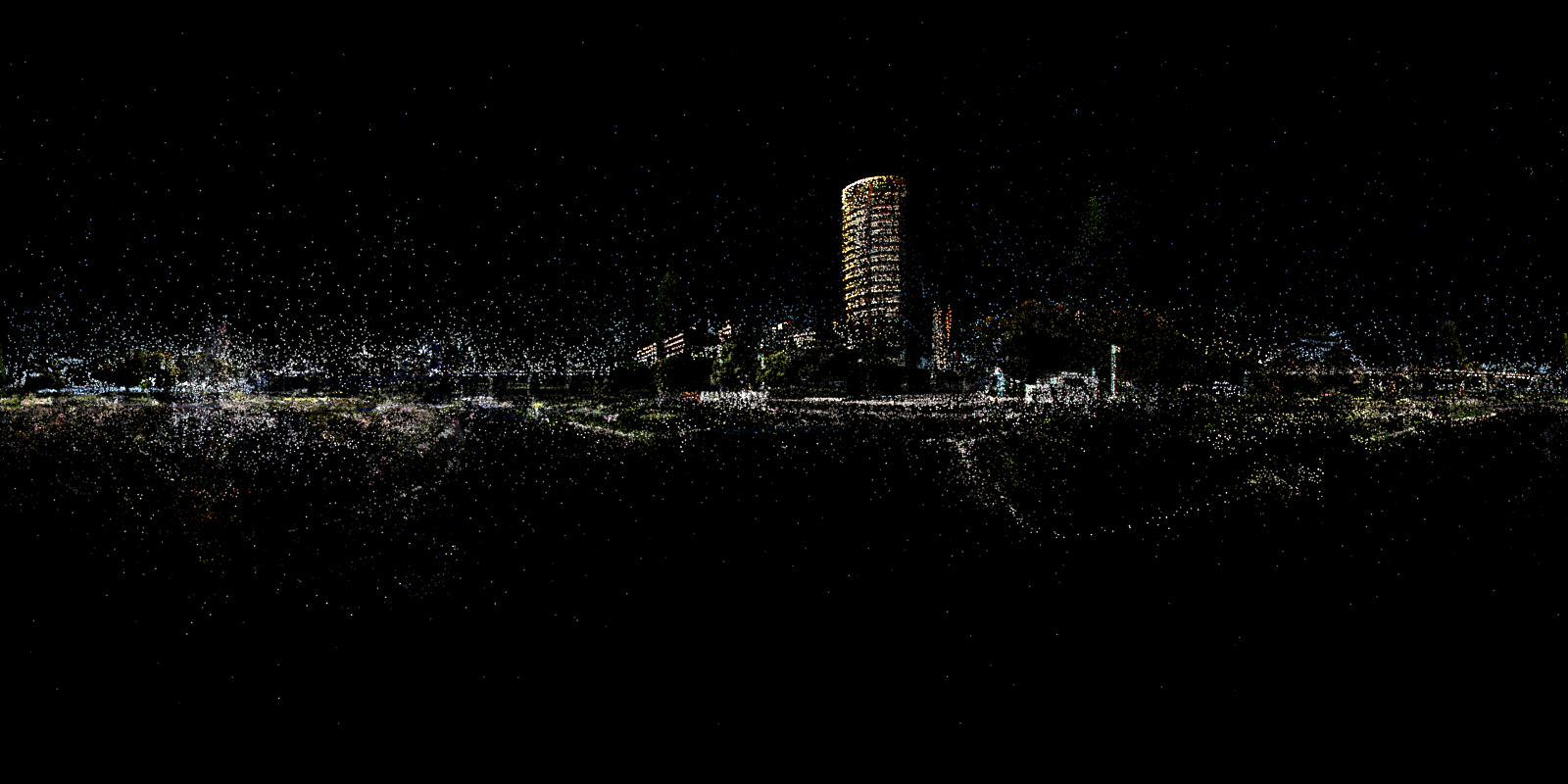
Scene #1	Scene #2

다음과 같은 과정을 통해 비슷하게 그릴 수 있다.

Near -> Far plane 으로 black background 에 pointcloud 만 loading 해서 rendering
Center (training camera 의 mean 으로 잡았음, 직접 설정해도 무방) 으로 부터 radius 를 키우면서 sphere 안의 splats 만 원래대로 rendering

마치며

알고리즘의 많은 부분을 MLP 에 맡기는 NeRF 의 경우, Linear Algebra 나 Computer Graphics 관점에서 코드가 어떻게 짜여져 있는지 분석하는 것이 쉬운 편인데, 3D Gaussian Splatting 의 경우 explicit 한 primitive 를 다루기 때문에 rasterization module 이 매우 섬세하게 설계되어 있어 수학적, 코드적 관점으로 분석하기 꽤나 난해한 것 같다.

이번 글은 inria group 의 diff-gaussian-rasterizer 의 forward 함수 위주로 분석하였는데, 실제 구현에는 Spherical Harmonics 로부터 RGB color 를 계산, CUDA thread block 할당 및 rasterization 과정에 대한 backward 또한 포함되어 있다. Backward 는 앞서 설명한 forward 계산의 역과정에 가까우며, forward step 에서 front-to-back 으로 탐색하는 것과 반대로 back-to-front 로 탐색하면서 gradient 를 계산한다.

~~기회가 된다면 gsplat 의 rasterizer 와 비교하는 글도 써보려고 한다.~~