잃어버린 3D Gaussian Splatting 의 Densification Strategy 를 찾아서... (feat. 3DGS-MCMC, AbsGS and TrimGS)

Hwan Heo·2024년 7월 21일

3D Gaussian Splatting AbsGS Adaptive Density Control Neural Rendering TrimGS markov chain monte carlo

Neural Rendering

목록 보기

14/16

이 글은

에 대한 간략한 review 가 포함되어 있습니다.

1. 들어가며

Recap. 3D Gaussian Splatting 의 Adaptive Density Control

Blog 에서 직접적으로 다룬 적은 없지만, 3D Gaussian Splatting 의 괄목할만한 성장과 View Synthesis 성능에는 적절한 학습 전략에 기인하는 바도 크다.

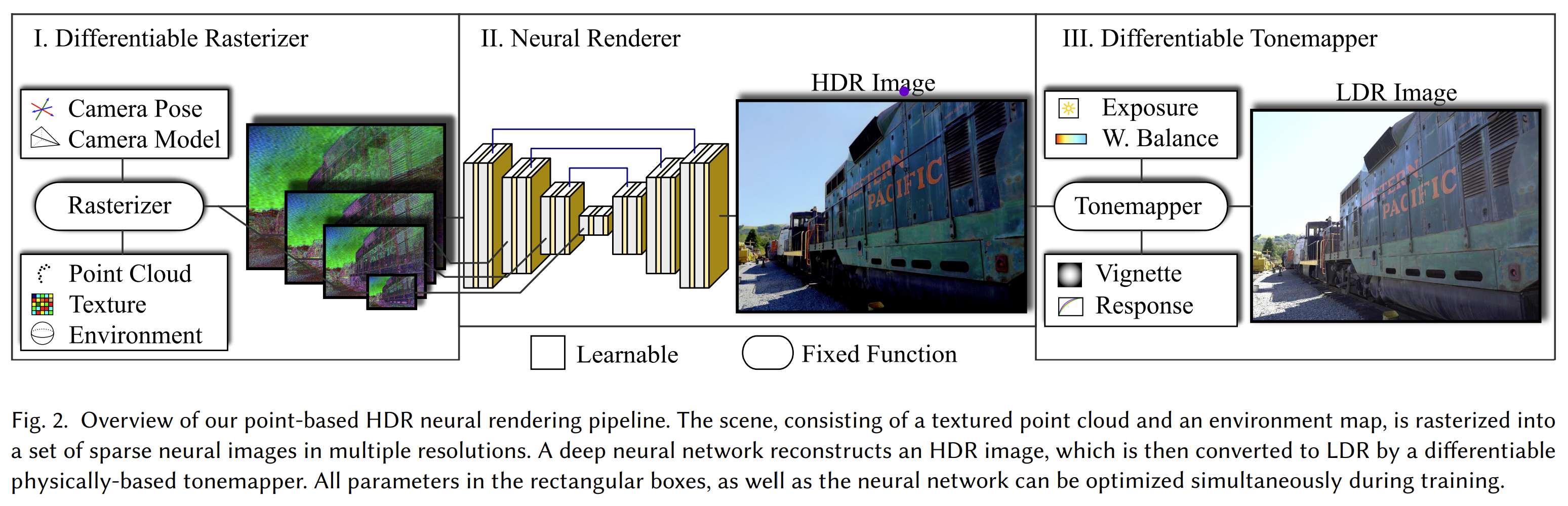
Dense pointcloud 를 3D scene 에서 활용하는 전략이야 이미 CG/CV 분야에서 예전부터 쓰이던 방법이며, 3D GS 발표 전 가장 3D GS 와 비슷한 알고리즘인 ADOP 에서도 SfM 을 통해 얻은 pointcloud 를 rasterize 하여 U-Net 구조의 Neural Renderer 에 이를 집어넣고 복각하는 알고리즘을 제시한 바 있다.

ADOP: Approximate Differentiable One-Pixel Point Rendering.

하지만 이들 방법과 가장 차별화되는 3D GS 만의 특징은 learnable 하게 scene 안의 Gaussian 들을 ‘move’, ‘split’, ‘clone’, ‘prune’ 하는, Adaptive Density Control 전략이다.

방법 자체는 매우 간단한데, differentiable rasterization 으로 개별 Gaussian 의 gradient 를 구할 수 있으므로 gradient threshold (hyperparameter) 를 넘는 Gaussian 에 대해,

Large Gaussian 의 경우, 1.6배 작은 2개의 Gaussian 으로 나누고 (split)
Small Gaussian 의 경우, gradient 방향으로 복제하며, (clone)
Opacity 가 threhold 이하인 경우엔 삭제하는 (prune)

일련의 전략들로 이루어져 있다.

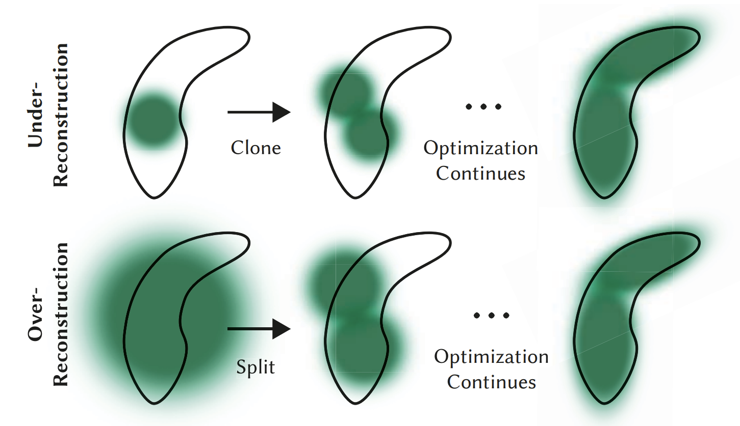
얼핏 생각하기에 Gradient 가 작은 Under / Over reconstruction 영역에 대해서 적절하게 Gaussian 을 나누고 추가하는 이상할 게 없는 전략이지만, ADC 에는 너무나도 많은 heuristic 이 존재한다. 애초에 전략의 설계 자체가 heuristic 이며, gradient threshold, size scaler, opacity threshold 등 수많은 hyperparameter 가 존재한다.

대체 왜? 3D GS 의 ADC 를 통해서 Gaussian 들을 추가하고 삭제해야 하는가? 더 적절한 Densification 전략은 없는가?

이 블로그 글을 통해 최근 발표되고 있는 3D GS densification 관련 논문들을 살펴보고, 이러한 질문에 대해 간략한 중간 답안을 정리해보려 한다.

2. 잃어버린 3D GS 의 Densification Strategy 를 찾아서

2.1. ADC 의 수학적 해석

ADC 에 이론적인 정당성과 수학적으로 조금 더 나은 설계를 보여주었던 논문 중에 가장 주목할만한 논문은 2024 NeurIPS 제출 paper 인 3D Gaussian Splatting as Markov Chain Monte Carlo 이다.

이 논문에서 저자들은 Set of 3D Gaussians 이 physical representation distribution (training images) 에 대한 random sample 이라고 간주할 수 있다고 주장한다, 즉 3D GS 자체를 아래 distribution 을 따르는 probability 에 대한 MCMC sample 이라고 보고,

\mathcal G \sim \mathcal P \propto e^{-{ \mathcal L}}

3D GS 학습은 이 probability 의 negative log likelihood 을 이용한 SGLD sampling process 로 해석한다.

g \leftarrow g + a \cdot \nabla_g \log P(g) + b \cdot \epsilon

where $a=-\lambda_{\text{lr}}, b=0$ .

이 해석을 이용하면 3D GS 의 Adaptive Density Control 은 MCMC framework 에서의 deterministic state transition 으로 간주할 수 있다. 즉, old gaussian -> new gaussian 으로 update 하는 ADC 는

\mathcal P (\mathcal G_{\text{old}} ) \simeq \mathcal P (\mathcal G_{\text{new}} )

MCMC sampling 에서 probability observation 을 보존하는 state transition 으로 해석할 수 있다.

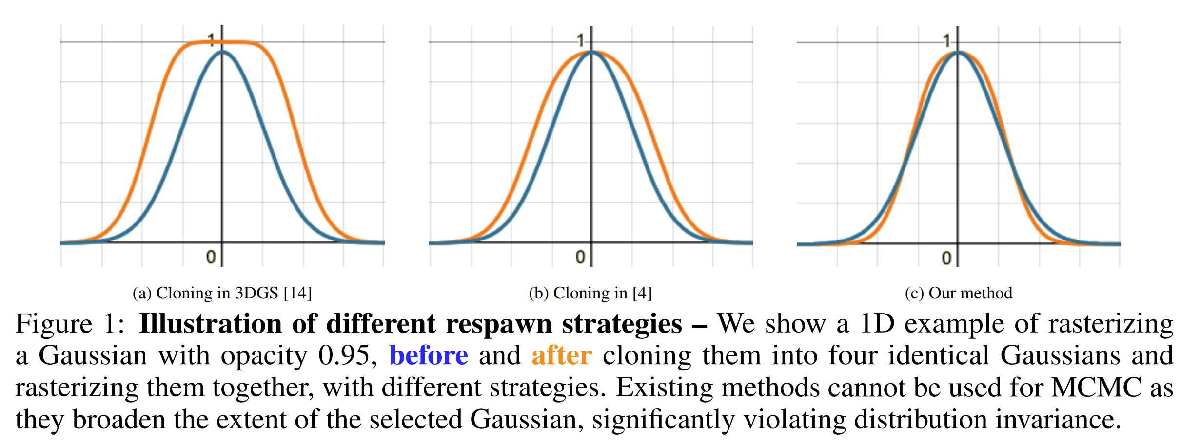
저자들은 $\mathcal P (\mathcal G_{\text{old}} ) \simeq \mathcal P (\mathcal G_{\text{new}} )$ 를 보장하기 위해, 기존 ADC 의 densification rule 을 일부 수정한 relocation rule 또한 제시한다.
구체적으로는 dead Gaussians 을 적절한 live Gaussians 으로 옮기는 method 인데, 다음과 같은 공식을 통해서 opacity 가 일정 값보다 낮은 Gaussian 을 prune 하는 대신, live 영역으로 relocate 하게 만든다.

\begin{aligned} \mu_{1, \ldots, N} & = \mu_{\text{old}}, \\ o_{1, \ldots, N} & = 1 - (1 - o_{\text{old}})^N, \\ \Sigma_{1, \ldots, N} & = (o_{\text{old}})^2 \left( \sum_{i=1}^N \sum_{k=0}^{i-1} \left( \binom{i-1}{k} (-1)^k \frac{(o_{\text{new}})^{k+1}}{k+1} \right) \right) - 2 \Sigma_{\text{old}}. \end{aligned}

(식에 대한 유도는 논문 Appendix 참조. old Gaussians 과 new Gaussians 의 central observation 이 같도록 하는 식을 approximation 하면 상기 공식이 유도된다.)

아래 1D example 을 통해서도 (a) ADC 와 (c) Relocation-MCMC 를 비교했을 때 MCMC 에서 제시된 방법이 probability 를 훨씬 잘 보존하는 것을 볼 수 있다.

그럼 이 논문 하나로 ADC 설명과 이에 대한 연구는 끝? 이면 좋겠지만... 당연히 그렇지 않다.

3D GS-MCMC 의 실제 구현은 dead Gaussian 전부를 live 로 relocate 하는 것에 그치지 않고, 일정 비율 (in official: 5%) 을 정해두고, opacity 에 따라 new Gaussian 을 sampling 하는 add new GS method 또한 활용한다.

	def add_new_gs(self, cap_max):
        current_num_points = self._opacity.shape[0]
        target_num = min(cap_max, int(1.05 * current_num_points))
        num_gs = max(0, target_num - current_num_points)

        if num_gs <= 0:
            return 0

        probs = self.get_opacity.squeeze(-1) 
        add_idx, ratio = self._sample_alives(probs=probs, num=num_gs)
        new_xyz = self._update_params(add_idx, ratio=ratio)

당연하겠지만 위에서 언급한 'Relocation' 만으로는 new Gaussian 을 추가하는 것이 불가능하기 때문에, under Reconstruction region 에 대해 다루기 위해 해당 전략을 사용하는 것이다. 이 method 는 opacity 를 PDF 로 sampling 해서 observation 이 달라지지는 않겠지만, 과연 Under Reconstruction Region 에 대해 적절하게 densification 이 일어날 것인가하는 의문이 있다.

또한 scene 마다 적절한 maximum particle number (cap_max) 를 정의해두어야 한다든가, 추가될 Gaussian 의 percentage (5%) 등 새로운 hyperparameter 이 많기 때문에 논문의 fancy함 만큼의 석연찮음 또한 남긴 방법이었다.

2.2. Gradient Threshold 로 거르는 거 진짜 좋나요?

3D GS-MCMC 의 relocation / add new GS 가 완벽한 해결책을 남긴 것은 아니지만, 그와 별개로 ADC 자체를 MCMC sampling 에서의 state transition 으로 해석할 수 있다는 수확이 있었다.

이 아래에서는 ADC 의 original densification 기조를 유지하되, gradient threshold 로 split / clone 될 Gaussian 을 고르는 ADC 를 수정할 것을 제시한 전략 두 가지를 소개한다.

2.2.1. AbsGS: Recovering Fine Details for 3D Gaussian Splatting

AbsGS 는 '그거 왜 다 더해요?' 로 요약할 수 있는 논문이다.

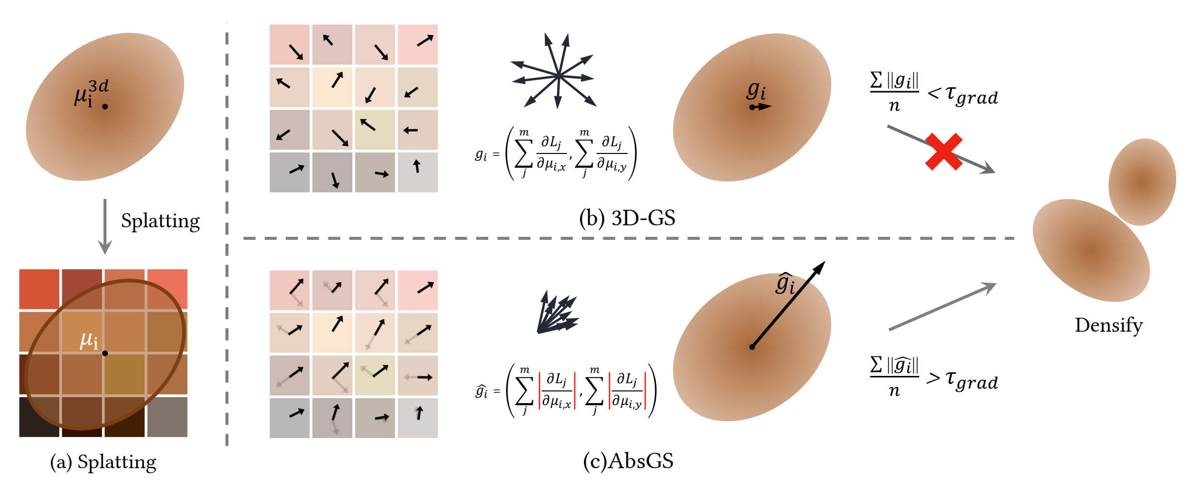
위의 그림에서 볼 수 있듯이 Large Gaussian 의 경우에는 tile-based rasterization 으로, tile-wise gradient 가 더해지면 전체 gradient magnitude 값이 작아지는 경우가 있어, ADC 적용 대상으로 선택되지 못하는 경우가 종종 있다.

따라서 단순히 tile-wise gradient (vector) 를 더하지 말고, tile-wise gradient homodirectional gradient 를 더해서 densification rule 로 삼자는 게 주요 아이디어이다. 실제 구현 자체도 이를 위해 kernel 수정이 딱 두 줄 (실제로는 좀 더 되긴 한다) 추가되어 있다.

backward kernel implementation

// Homodirectional Gradient
atomicAdd(&dL_dmean2D[global_id].z, fabs(dL_dG * dG_ddelx * ddelx_dx));
atomicAdd(&dL_dmean2D[global_id].w, fabs(dL_dG * dG_ddely * ddely_dy));

이를 통해 기존 ADC 로는 잘 선택되지 않는 large gaussian 도 ADC 의 적용 대상으로 선택할 수 있다고 주장한다.

아래 figure (d), (e) 는 각각 original ADC, absGS 로 선택된 Gaussian 들을 시각화 한 것인데, large Gaussian 들의 경우 실제로 AbsGS 의 전략을 통해 훨씬 densification 대상에 잘 선택되는 것을 볼 수 있다.

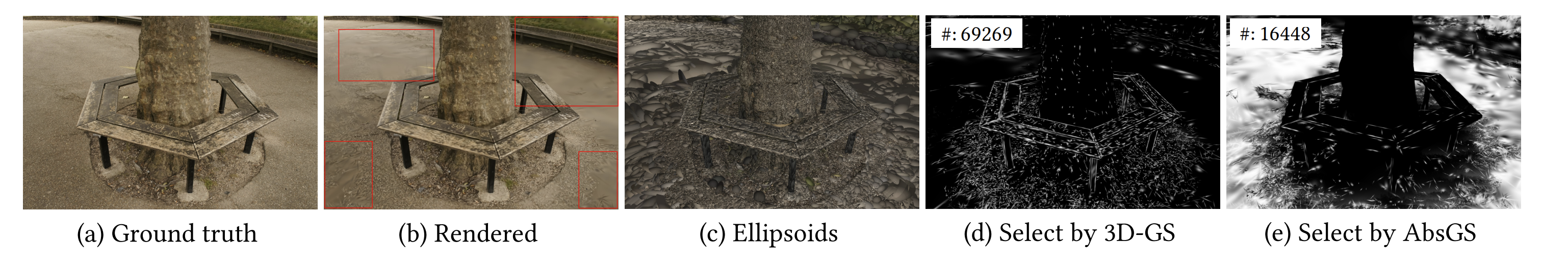
실제 구현에서는 cloning 단계에서는 기존 ADC 의 방법을 따르고, split 단계에서만 이러한 absolute gradient 를 이용하는 방식을 취하고 있다.

    def densify_and_prune(self, max_grad, max_grad_abs, min_opacity, extent, max_screen_size):
        grads = self.xyz_gradient_accum / self.denom
        grads[grads.isnan()] = 0.0

        grads_abs = self.xyz_gradient_accum_abs / self.denom
        grads_abs[grads_abs.isnan()] = 0.0

        self.densify_and_clone(grads, max_grad, extent)
        self.densify_and_split(grads_abs, max_grad_abs, extent)
        
        ...

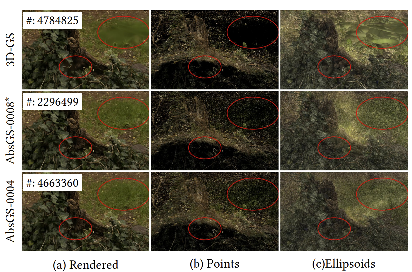
3D GS 를 실제로 학습시켜보면, observation 이 떨어지는 영역에 대해서 densify 가 많이 일어나지 않아 blurry 하게 scene 이 복각되는 모습이 많은데, AbsGS 를 이용하면 이러한 모습이 많이 개선된다.

2.2.2. TrimGS: Gaussian Splatting for Accurate Geometry Representation

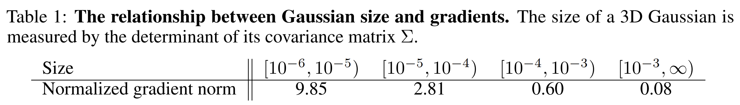
TrimGS 또한 AbsGS 와 굉장히 비슷한 관찰, 'large gaussian 의 gradient 가 매우 noisy 할 것' 임을 예상하고 논리를 전개한다.

논문에 제시된 아래 table 에서, Gaussian 의 크기가 클수록 gradient 값이 작아지는 것을 볼 수 있다. (AbsGS 와 동일한 관찰)

대신에 original ADC, AbsGS 와는 다르게 Gaussian compression 등에서 사용하는 'Contribution' 의 개념으로 ADC rule 을 제시한다.

하기 공식은 alpha-blending weight 로써 일종의 single-view contribution 값으로도 해석할 수 있는데,

C_k = \sum_{p \in \mathcal{P}_k} \alpha_i(p) \prod_{j=1}^{i(p)-1} (1 - \alpha_j)

이 값을 통해 contribution 을 계산하면 gradient 와는 반대로 large gaussian 은 높게, small gaussian 은 낮게 나올 것이다.

따라서 이를 일반화하여 ADC 를 위한 contribution 공식을 다음과 같이 제안한다.

C_k = \frac{1}{|\mathbb{P}_k|} \sum_{p \in \mathcal{P}_k} \left( \alpha_i(p) \right)^\gamma \left( \prod_{j=1}^{i(p)-1} (1 - \alpha_j) \right)^{(1 - \gamma)}

여기서 $\mathbb{P}_k$ 는 projected area 에 투영된 pixel 의 갯수이다. 즉 project view 에 대한 contribution 을 측정하되, 이를 pixel number 로 normalize 하여 large / small gaussian 의 태생적인 contribution 차이를 줄인다.

또한 저자들은 $\gamma$ 의 도입에 대해서도 다음과 같은 이유를 들어 설명한다.

$\gamma$ 가 커질수록 accumulated transmiattance 대신 opacity 에 가중치가 크게 되어, opacity-based pruning 인 original ADC 에 가까워진다.
Surface 를 벗어난 Gaussian 들이 부정확한 geometry 를 가지기 때문에, surface outside 에서는 transmittance 가 부각되고, inner 에서는 opacity 가 부각되어 조금 더 정확한 geometry 를 가질 수 있을 것이다.

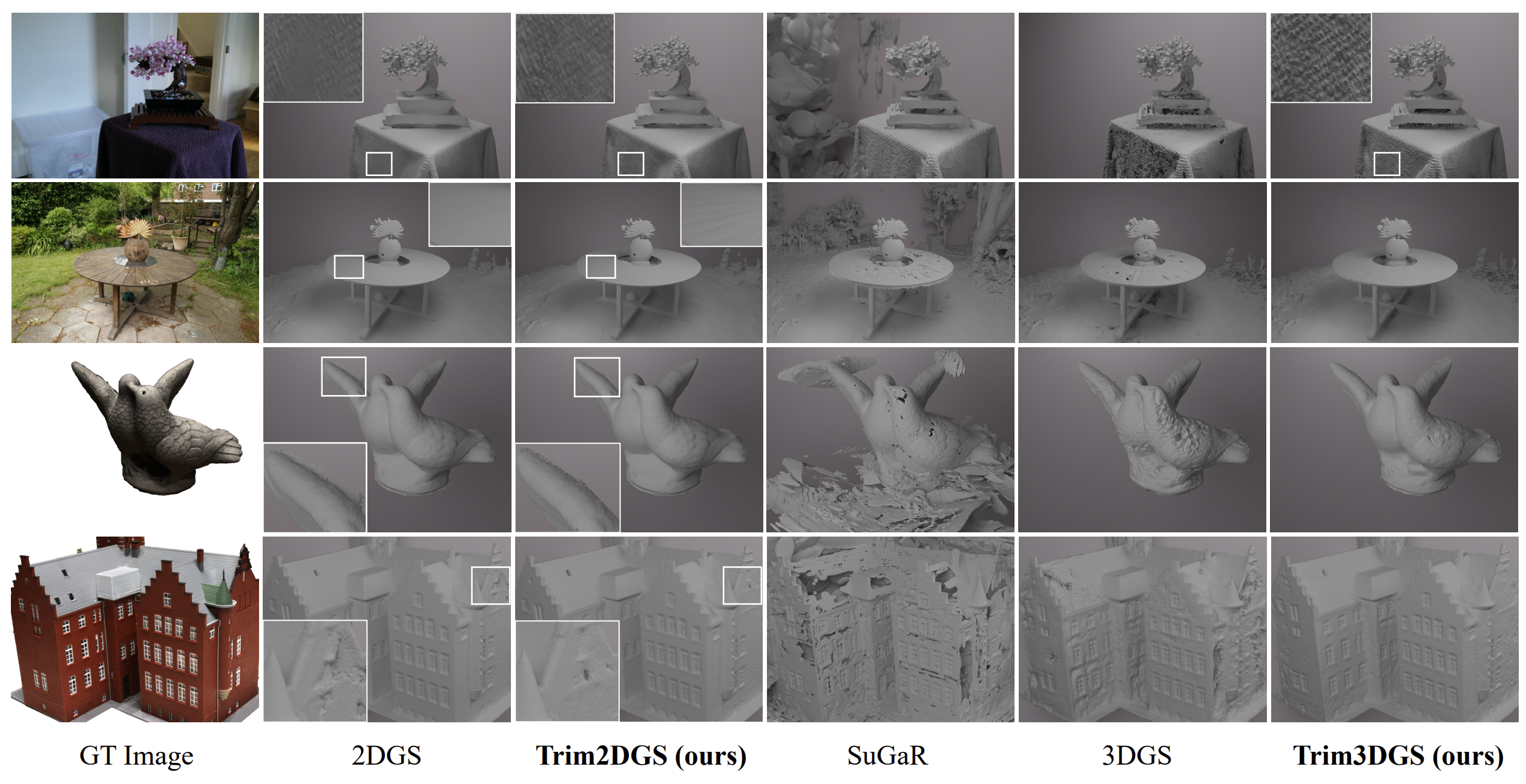
실제 구현에서는 Vanilla 3D GS, 2D GS 를 학습한 후 추가 7K iteration 동안 상기 contribution 을 통한 trimming 전략을 실행하도록 구성되어 있다. 실제로 알고리즘을 실험해봤을 때나, 논문의 정성적/정량적 결과를 비교해도 original ADC 대비 좋은 모습을 보여주기는 하지만 조금 더 공정한 비교를 위해서는 Vanilla 3D GS / 2D GS 는 23K 학습 이후 TrimGS 7K tune 으로 실험했어야 공정한 게 아닌가하는 생각이 있다.

3. 마치며

이 글에서는 3D Gaussian Splatting 과 관련된 세 가지 논문을 통해 Adaptive Density Control 의 중요성과 최근 발전 동향을 살펴보았다. 3D GS-MCMC 에서는 ADC 의 수학적인 해석, 또한 state transition 을 위한 적절한 relocation 전략을, AbsGS 와 TrimGS 에서는 기존 ADC 가 잘 다루지 못하던 large gaussian 의 blurry reconstruction 문제를 해결하는 방법들이 제시되었다.

하지만 아직도 각 방법들의 heuristicity 가 크며, scene 의 종류에 따라 hyperparameter tunning 해야하는 문제가 남아있기 때문에 3D GS 의 densification 전략에 대한 연구도 지속적으로 나올 것이라 예상한다.

(여담으로 마치며를 쓰기 귀찮아서 ChatGPT 에게 맡겼는데... 걍 요약만 해주길래 prompt 로 future work 써달라고 부탁할까 하다가 그냥 짧게 내가 썼다 ㅠ)