
챌린지 주제
AI를 통해 네트워크에서 발생한 이상징후를 탐지하는 것
데이터셋: 네트워크 로그 데이터셋
train.csv
ts: 타임스탬프uid: 커넥션IDid.orig_h: 출발지IP주소(경연데이터에는 미포함)id.orig_p: 출발지TCP/UDP포트id.resp_h: 도착지IP주소(경연 데이터에는 미포함)id.resp_p: 도착지TCP/UDP포트proto: TCP레이어 프로토콜service: 동적으로 탐지된 애플리케이션 프로토콜(있는 경우에만)duration: 패킷 연결 지속 시간orig_bytes: TCP인 경우,시퀀스 넘버로 구한 출발지 페이로드 바이트resp_bytes: TCP인 경우,시퀀스 넘버로 구한 도착지 페이로드 바이트conn_state: 연결 상태
- S0: 연결 시도는 보이나,응답 없음
- S1: 연결이 성립되었지만,종료되지 않음
- SF: 정상적인 연결&종료
- REJ: 연결 시도 거부됨
- S2: 연결됨.출발지에서 종료 요청을 했으나 응답이 없는 상태
- S3: 연결됨.도착지에서 종료 요청을 했으나,응답이 없는 상태
- RSTO: 연결됨.출발지 연결 종료(RST)
- RSTR: 연결됨.도착지 연결 종료(RST)
- RSTOSO: 출발지에서SYN, RST순서로 패킷 전송(응답은 아직X)
- RSTRH: 도착지에서RYN, RST순서로 패킷 전송(응답은 아직X)
- SH: 출발지에서SYN, FIN순서로 패킷 전송(응답은 아직X) (half-open)
- SHR: 도착지에서SYN, ACK, FIN순서로 패킷 전송(응답은 아직X)
- OTH: SYN도 없고,연결도 닫히지 않은 상태.스트림 트래픽 전송 중
local_orig: 로컬 연결인 경우T,원격 연결인 경우Flocal_resp: 로컬 연결인 경우T,원격 연결인 경우Fmissed_bytes: 컨텐츠 갭 내의 분실 바이트 개수history: 연결 상태 히스토리
- S: ACK가 세트되지 않은SYN
- H: SYN-ACK
- A: 순수ACK
- D: 페이로드를 담고 있는 패킷
- F: FIN이 세트된 패킷
- R: RST가 세트된 패킷
- C: 잘못된 체크섬 값을 가진 패킷
- I: 일관되지 않은 패킷
orig_pkts: 출발지 패킷의 개수orig_ip_bytes: 출발지IP바이트의 개수resp_pkts: 목적지 패킷의 개수resp_ip_bytes: 목적지IP바이트의 개수tunnel_parents: 터널링이 적용된 경우,부모 캡슐의 연결UIDclass: 악성 트래픽 여부(1은 악성, 0은 정상)(경연 데이터에는 미포함)
데이터 분석
데이터 분석 단계에서는 경연에 미포함되는 feature는 다루지 않도록 하겠다.
# AI기반 네트워크 위협탐지 미니 챌린지

import pandas as pd

# 데이터 불러오기
train = pd.read_csv('train.csv')
test = pd.read_csv('test.csv')
answer = pd.read_csv('answer.csv')

train.shape, test.shape, answer.shape
((19735, 23), (1631, 21), (1631, 2))우선 pandas라이브러리를 이용해 데이터셋을 로드했다.
학습 데이터셋의 데이터 개수는 총 19735개, 경연 데이터셋의 데이터 수는 총 1631개이다.
학습 데이터셋의 class분포를 살펴보자.
# 데이터 시각화

import matplotlib.pyplot as plt

# 데이터 분포 확인
# 정상과 악성의 분포 확인

plt.figure(figsize=(5, 5))
plt.title('class distribution')
plt.bar(train['class'].unique(), train['class'].value_counts(), width=0.4, color=['skyblue', 'pink'])
plt.xticks(train['class'].unique())
plt.xlabel('class (0: normal, 1: malicious)')
plt.ylabel('count')
plt.show()

print(train['class'].value_counts())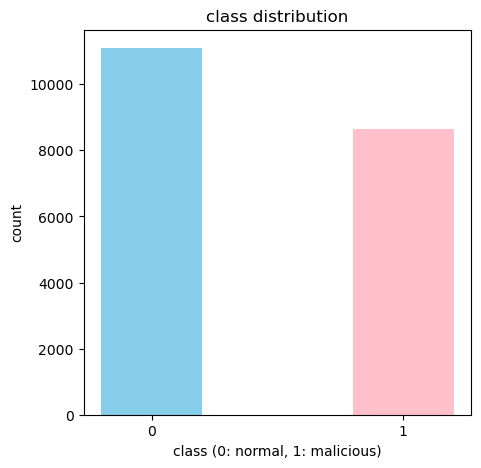
class
0.0    11096
1.0     8639
Name: count, dtype: int64
정상 데이터는 11096개, 악성 데이터는 8639개이다. 정상 데이터와 악성 데이터의 분포가 어느 한쪽으로 크게 치우치지 않았기 때문에 데이터의 불균형으로 인한 학습 저해 현상은 없을 것으로 판단했다.
다음은 class 별 id.orig_p과 id.resp_p의 분포이다.
# class 별 데이터 분포 확인
# class 별 id.orig_p의 분포 확인

plt.figure(figsize=(5, 5))
plt.title('id.orig_p distribution')
plt.hist(train[train['class'] == 0]['id.orig_p'], color='skyblue', label='normal', alpha=0.5)
plt.hist(train[train['class'] == 1]['id.orig_p'], color='pink', label='malicious', alpha=0.5)
plt.legend()
plt.xlabel('id.orig_p')
plt.ylabel('count')
plt.show()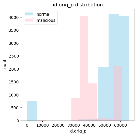
# class 별 id.resp_p의 분포 확인

plt.figure(figsize=(5, 5))
plt.title('id.resp_p distribution')
plt.hist(train[train['class'] == 0]['id.resp_p'], color='skyblue', label='normal', alpha=0.5)
plt.hist(train[train['class'] == 1]['id.resp_p'], color='pink', label='malicious', alpha=0.5)
plt.legend()
plt.xlabel('id.resp_p')
plt.ylabel('count')
plt.show()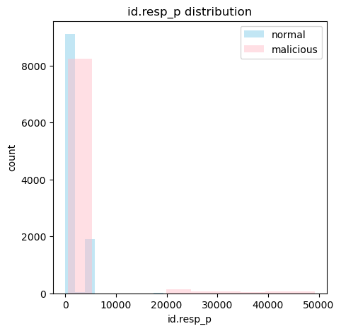
두 feature모두 정상과 악성에 따라서 어느정도 분포가 나뉘는 걸 확인할 수 있다.
다음은 proto의 분포를 확인해보자.
# class 별 proto 분포 시각화 with pandas

train.groupby('class')['proto'].value_counts().plot(kind='bar', figsize=(5, 5), color=['skyblue', 'pink', 'lightgreen'], alpha=0.5, rot=0)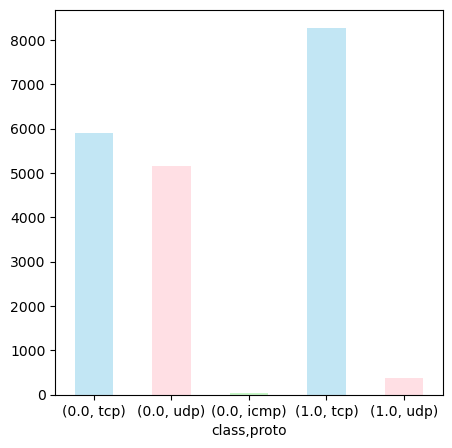
정상 트래픽의 경우 tcp와 udp, 그리고 조금의 icmp로 구성되어 있지만 악성 트래픽의 경우 거의 대부분의 데이터가 tcp인 것을 확인할 수 있다.
다음은 service의 분포를 확인해보자.
# class 별 service 분포 시각화 with pandas

train.groupby('class')['service'].value_counts().plot(kind='bar', figsize=(5, 5), color=['skyblue', 'pink', 'lightgreen'], alpha=0.5, rot=45)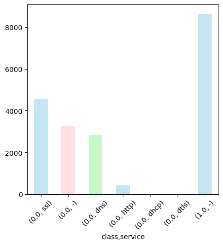
다음은 duration의 분포를 확인해보자. 먼저 duration의 분포를 확인하기 전에 해줘야 할 작업이 있다. duration은 패킷 연결 지속 시간을 뜻하는데 데이터를 확인해보면 -값으로 채워진 데이터들이 많다. 해당 데이터들의 개수를 확인해보자.
# duration의 값이 '-'인 데이터 개수 확인

len(train[train['duration'] == '-'])271확인해보니 271개의 데이터가 있었다. 패킷 연결 지속 시간이기 때문에 -값은 연결이 지속되지 않았다는 의미로 간주하고 모두 0으로 바꿔주도록 하자.
# duration이 '-'인 데이터의 duration을 0으로 변경

train.loc[train['duration'] == '-', 'duration'] = 0
len(train[train['duration'] == '-'])0변경 완료 후 시각화를 진행해주었다.
# duration 데이터 타입 변경 후 시각화

train['duration'] = train['duration'].astype('float64')

plt.figure(figsize=(5, 5))
plt.title('duration distribution')
plt.hist(train[train['class'] == 0]['duration'], color='skyblue', label='normal', alpha=0.5)
plt.hist(train[train['class'] == 1]['duration'], color='pink', label='malicious', alpha=0.5)
plt.legend()
plt.xlabel('duration')
plt.ylabel('count')
plt.show()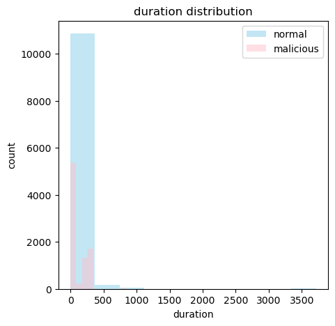
duration의 데이터 타입이 object였기 때문에 시각화하는 데에 어려움이 있어서 float64형으로 형변환 후 시각화 해주었다. duration역시 어느정도 분포의 패턴이 보이는것을 확인할 수 있다. 하지만 데이터의 편차가 너무 크기 때문에 전처리 단계에서 feature로 사용하기 위해서는 스케일링을 진행해주어야 하는 데이터로 판단하였다.
위와 같이 모든 feature들에 대하여 시각화를 통한 데이터 분석을 진행한 후 최종적으로 판단한 결과, 학습에 도움이 되지 않는 feature는 Unnamed: 0, ts, uid, id.orig_h, id.resp_h, tunnel_parents라고 판단하였다. 이유는 다음과 같다.
Unnamed: 0: 단순 인덱스 데이터ts: 시계열 분석을 하지 않는 이상 학습에 쓰기 어려운 데이터uid: 커넥션들의 고유ID 데이터id.orig_h: 경연 미포함 데이터id.resp_h: 경연 미포함 데이터tunnel_parents: 모든 값이(empty)로 동일한 데이터
따라서, 데이터 전처리 단계에서 해당 feature들은 제거 후 진행하기로 하였다.
데이터 전처리
# 데이터 모양 확인

train| Unnamed: 0 | ts | uid | id.orig_h | id.orig_p | id.resp_h | id.resp_p | proto | service | duration | ... | local_orig | local_resp | missed_bytes | history | orig_pkts | orig_ip_bytes | resp_pkts | resp_ip_bytes | tunnel_parents | class | |
|---|---|---|---|---|---|---|---|---|---|---|---|---|---|---|---|---|---|---|---|---|---|
| 0 | 0 | 1632859201.94749 | CPNl6k3JbVOG4tz1Zd | 192.168.87.131 | 60615.0 | 192.168.87.2 | 53.0 | udp | dns | 0.270559 | ... | T | T | 0.0 | Dd | 1.0 | 62.0 | 1.0 | 137.0 | (empty) | 0.0 |
| 1 | 1 | 1632859159.2100391 | COUSXg4wGYe6luWFG8 | fe80::20c:29ff:fe9f:ebb | 133.0 | ff02::2 | 134.0 | icmp | - | - | ... | F | F | 0.0 | - | 1.0 | 56.0 | 0.0 | 0.0 | (empty) | 0.0 |
| 2 | 2 | 1632859214.3695712 | CuEEhk3Wt5ChCk2U6f | 192.168.87.131 | 55924.0 | 192.168.87.2 | 53.0 | udp | dns | 0.023672 | ... | T | T | 0.0 | Dd | 1.0 | 70.0 | 1.0 | 177.0 | (empty) | 0.0 |
| 3 | 3 | 1632859214.400497 | CEEAX035N9QYuH3Xq5 | 192.168.87.131 | 54692.0 | 192.168.87.2 | 53.0 | udp | dns | 0.018691 | ... | T | T | 0.0 | Dd | 1.0 | 71.0 | 1.0 | 178.0 | (empty) | 0.0 |
| 4 | 4 | 1632859214.424631 | Cml68B12Tm1BNYtiBl | 192.168.87.131 | 37227.0 | 192.168.87.2 | 53.0 | udp | dns | 0.002733 | ... | T | T | 0.0 | Dd | 1.0 | 73.0 | 1.0 | 128.0 | (empty) | 0.0 |
| ... | ... | ... | ... | ... | ... | ... | ... | ... | ... | ... | ... | ... | ... | ... | ... | ... | ... | ... | ... | ... | ... |
| 19730 | 3525 | 1632937604.975284 | Ck9Vxk3npjUeqwmjC6 | 20.20.20.100 | 65216.0 | 203.217.236.19 | 443.0 | tcp | ssl | 0.012203 | ... | T | F | 3754.0 | ShADacFr | 6.0 | 776.0 | 5.0 | 204.0 | (empty) | 0.0 |
| 19731 | 3526 | 1632937553.091704 | CURubA6OnYIs9UFQ1 | 192.168.87.130 | 54735.0 | 216.58.220.110 | 443.0 | udp | - | 0.204099 | ... | T | F | 0.0 | Dd | 9.0 | 3875.0 | 10.0 | 4356.0 | (empty) | 0.0 |
| 19732 | 3527 | 1632937553.091831 | CrmjFs1glyZyU4aQwg | 20.20.20.100 | 54735.0 | 216.58.220.110 | 443.0 | udp | - | 0.204107 | ... | T | F | 0.0 | Dd | 9.0 | 3875.0 | 10.0 | 4356.0 | (empty) | 0.0 |
| 19733 | 3528 | 1632937540.984622 | C0yAyZ1EYy1KC50ovl | 192.168.87.130 | 55672.0 | 8.8.4.4 | 443.0 | udp | - | 18.059633 | ... | T | F | 0.0 | Dd | 22.0 | 3821.0 | 28.0 | 8203.0 | (empty) | 0.0 |
| 19734 | 3529 | 1632937540.9848368 | C6wugh1Lw2m6sgXwqi | 20.20.20.100 | 55672.0 | 8.8.4.4 | 443.0 | udp | - | 18.059590 | ... | T | F | 0.0 | Dd | 22.0 | 3821.0 | 28.0 | 8203.0 | (empty) | 0.0 |
19735 rows × 23 columns
학습에 사용하지 않을 데이터부터 제거하자.
# 1. 학습 미사용 데이터 제거 (Unnamed: 0, ts, uid, id.orig_h, id.resp_h, tunnel_parents)

train.drop(['Unnamed: 0', 'ts', 'uid', 'id.orig_h', 'id.resp_h', 'tunnel_parents'], axis=1, inplace=True)
train| id.orig_p | id.resp_p | proto | service | duration | orig_bytes | resp_bytes | conn_state | local_orig | local_resp | missed_bytes | history | orig_pkts | orig_ip_bytes | resp_pkts | resp_ip_bytes | class | |
|---|---|---|---|---|---|---|---|---|---|---|---|---|---|---|---|---|---|
| 0 | 60615.0 | 53.0 | udp | dns | 0.270559 | 34 | 109 | SF | T | T | 0.0 | Dd | 1.0 | 62.0 | 1.0 | 137.0 | 0.0 |
| 1 | 133.0 | 134.0 | icmp | - | - | - | - | OTH | F | F | 0.0 | - | 1.0 | 56.0 | 0.0 | 0.0 | 0.0 |
| 2 | 55924.0 | 53.0 | udp | dns | 0.023672 | 42 | 149 | SF | T | T | 0.0 | Dd | 1.0 | 70.0 | 1.0 | 177.0 | 0.0 |
| 3 | 54692.0 | 53.0 | udp | dns | 0.018691 | 43 | 150 | SF | T | T | 0.0 | Dd | 1.0 | 71.0 | 1.0 | 178.0 | 0.0 |
| 4 | 37227.0 | 53.0 | udp | dns | 0.002733 | 45 | 100 | SF | T | T | 0.0 | Dd | 1.0 | 73.0 | 1.0 | 128.0 | 0.0 |
| ... | ... | ... | ... | ... | ... | ... | ... | ... | ... | ... | ... | ... | ... | ... | ... | ... | ... |
| 19730 | 65216.0 | 443.0 | tcp | ssl | 0.012203 | 524 | 3754 | RSTR | T | F | 3754.0 | ShADacFr | 6.0 | 776.0 | 5.0 | 204.0 | 0.0 |
| 19731 | 54735.0 | 443.0 | udp | - | 0.204099 | 3623 | 4076 | SF | T | F | 0.0 | Dd | 9.0 | 3875.0 | 10.0 | 4356.0 | 0.0 |
| 19732 | 54735.0 | 443.0 | udp | - | 0.204107 | 3623 | 4076 | SF | T | F | 0.0 | Dd | 9.0 | 3875.0 | 10.0 | 4356.0 | 0.0 |
| 19733 | 55672.0 | 443.0 | udp | - | 18.059633 | 3205 | 7419 | SF | T | F | 0.0 | Dd | 22.0 | 3821.0 | 28.0 | 8203.0 | 0.0 |
| 19734 | 55672.0 | 443.0 | udp | - | 18.059590 | 3205 | 7419 | SF | T | F | 0.0 | Dd | 22.0 | 3821.0 | 28.0 | 8203.0 | 0.0 |
19735 rows × 17 columns
결측치를 확인하고 제거하자.
# 2. 결측치 확인

train[train.isnull().any(axis=1)]| id.orig_p | id.resp_p | proto | service | duration | orig_bytes | resp_bytes | conn_state | local_orig | local_resp | missed_bytes | history | orig_pkts | orig_ip_bytes | resp_pkts | resp_ip_bytes | class | |
|---|---|---|---|---|---|---|---|---|---|---|---|---|---|---|---|---|---|
| 12352 | NaN | NaN | NaN | NaN | NaN | NaN | NaN | NaN | NaN | NaN | NaN | NaN | NaN | NaN | NaN | NaN | 0.0 |
| 16204 | NaN | NaN | NaN | NaN | NaN | NaN | NaN | NaN | NaN | NaN | NaN | NaN | NaN | NaN | NaN | NaN | 0.0 |
# 결측치 제거

train.dropna(inplace=True)
train[train.isnull().any(axis=1)]| id.orig_p | id.resp_p | proto | service | duration | orig_bytes | resp_bytes | conn_state | local_orig | local_resp | missed_bytes | history | orig_pkts | orig_ip_bytes | resp_pkts | resp_ip_bytes | class |
|---|
결측치를 성공적으로 제거하였으니 이제 각 feature별로 적절한 방법을 사용해 전처리를 진행한다.
id.orig_p,id.resp_p
# 3. id.orig_p, id.resp_p 전처리, 포트 정보이므로 int형으로 변경

train['id.orig_p'] = train['id.orig_p'].astype('int64')
train['id.resp_p'] = train['id.resp_p'].astype('int64')
train| id.orig_p | id.resp_p | proto | service | duration | orig_bytes | resp_bytes | conn_state | local_orig | local_resp | missed_bytes | history | orig_pkts | orig_ip_bytes | resp_pkts | resp_ip_bytes | class | |
|---|---|---|---|---|---|---|---|---|---|---|---|---|---|---|---|---|---|
| 0 | 60615 | 53 | udp | dns | 0.270559 | 34 | 109 | SF | T | T | 0.0 | Dd | 1.0 | 62.0 | 1.0 | 137.0 | 0.0 |
| 1 | 133 | 134 | icmp | - | - | - | - | OTH | F | F | 0.0 | - | 1.0 | 56.0 | 0.0 | 0.0 | 0.0 |
| 2 | 55924 | 53 | udp | dns | 0.023672 | 42 | 149 | SF | T | T | 0.0 | Dd | 1.0 | 70.0 | 1.0 | 177.0 | 0.0 |
| 3 | 54692 | 53 | udp | dns | 0.018691 | 43 | 150 | SF | T | T | 0.0 | Dd | 1.0 | 71.0 | 1.0 | 178.0 | 0.0 |
| 4 | 37227 | 53 | udp | dns | 0.002733 | 45 | 100 | SF | T | T | 0.0 | Dd | 1.0 | 73.0 | 1.0 | 128.0 | 0.0 |
| ... | ... | ... | ... | ... | ... | ... | ... | ... | ... | ... | ... | ... | ... | ... | ... | ... | ... |
| 19730 | 65216 | 443 | tcp | ssl | 0.012203 | 524 | 3754 | RSTR | T | F | 3754.0 | ShADacFr | 6.0 | 776.0 | 5.0 | 204.0 | 0.0 |
| 19731 | 54735 | 443 | udp | - | 0.204099 | 3623 | 4076 | SF | T | F | 0.0 | Dd | 9.0 | 3875.0 | 10.0 | 4356.0 | 0.0 |
| 19732 | 54735 | 443 | udp | - | 0.204107 | 3623 | 4076 | SF | T | F | 0.0 | Dd | 9.0 | 3875.0 | 10.0 | 4356.0 | 0.0 |
| 19733 | 55672 | 443 | udp | - | 18.059633 | 3205 | 7419 | SF | T | F | 0.0 | Dd | 22.0 | 3821.0 | 28.0 | 8203.0 | 0.0 |
| 19734 | 55672 | 443 | udp | - | 18.059590 | 3205 | 7419 | SF | T | F | 0.0 | Dd | 22.0 | 3821.0 | 28.0 | 8203.0 | 0.0 |
19733 rows × 17 columns
proto
# 4. proto 전처리 - one-hot encoding

from sklearn.preprocessing import OneHotEncoder

proto_ohe = OneHotEncoder(sparse=False)
proto_ohe.fit(train[['proto']])
proto_ohe_df = pd.DataFrame(proto_ohe.transform(train[['proto']]), columns=proto_ohe.categories_[0], index=train.index)
train = pd.concat([train, proto_ohe_df], axis=1)
train.drop(['proto'], axis=1, inplace=True)
train| id.orig_p | id.resp_p | service | duration | orig_bytes | resp_bytes | conn_state | local_orig | local_resp | missed_bytes | history | orig_pkts | orig_ip_bytes | resp_pkts | resp_ip_bytes | class | icmp | tcp | udp | |
|---|---|---|---|---|---|---|---|---|---|---|---|---|---|---|---|---|---|---|---|
| 0 | 60615 | 53 | dns | 0.270559 | 34 | 109 | SF | T | T | 0.0 | Dd | 1.0 | 62.0 | 1.0 | 137.0 | 0.0 | 0.0 | 0.0 | 1.0 |
| 1 | 133 | 134 | - | - | - | - | OTH | F | F | 0.0 | - | 1.0 | 56.0 | 0.0 | 0.0 | 0.0 | 1.0 | 0.0 | 0.0 |
| 2 | 55924 | 53 | dns | 0.023672 | 42 | 149 | SF | T | T | 0.0 | Dd | 1.0 | 70.0 | 1.0 | 177.0 | 0.0 | 0.0 | 0.0 | 1.0 |
| 3 | 54692 | 53 | dns | 0.018691 | 43 | 150 | SF | T | T | 0.0 | Dd | 1.0 | 71.0 | 1.0 | 178.0 | 0.0 | 0.0 | 0.0 | 1.0 |
| 4 | 37227 | 53 | dns | 0.002733 | 45 | 100 | SF | T | T | 0.0 | Dd | 1.0 | 73.0 | 1.0 | 128.0 | 0.0 | 0.0 | 0.0 | 1.0 |
| ... | ... | ... | ... | ... | ... | ... | ... | ... | ... | ... | ... | ... | ... | ... | ... | ... | ... | ... | ... |
| 19730 | 65216 | 443 | ssl | 0.012203 | 524 | 3754 | RSTR | T | F | 3754.0 | ShADacFr | 6.0 | 776.0 | 5.0 | 204.0 | 0.0 | 0.0 | 1.0 | 0.0 |
| 19731 | 54735 | 443 | - | 0.204099 | 3623 | 4076 | SF | T | F | 0.0 | Dd | 9.0 | 3875.0 | 10.0 | 4356.0 | 0.0 | 0.0 | 0.0 | 1.0 |
| 19732 | 54735 | 443 | - | 0.204107 | 3623 | 4076 | SF | T | F | 0.0 | Dd | 9.0 | 3875.0 | 10.0 | 4356.0 | 0.0 | 0.0 | 0.0 | 1.0 |
| 19733 | 55672 | 443 | - | 18.059633 | 3205 | 7419 | SF | T | F | 0.0 | Dd | 22.0 | 3821.0 | 28.0 | 8203.0 | 0.0 | 0.0 | 0.0 | 1.0 |
| 19734 | 55672 | 443 | - | 18.059590 | 3205 | 7419 | SF | T | F | 0.0 | Dd | 22.0 | 3821.0 | 28.0 | 8203.0 | 0.0 | 0.0 | 0.0 | 1.0 |
19733 rows × 19 columns
service
# 5. service 전처리 - one-hot encoding

service_ohe = OneHotEncoder(sparse=False)
service_ohe.fit(train[['service']])
service_ohe_df = pd.DataFrame(service_ohe.transform(train[['service']]), columns=service_ohe.categories_[0], index=train.index)
train = pd.concat([train, service_ohe_df], axis=1)
train.drop(['service'], axis=1, inplace=True)
train| id.orig_p | id.resp_p | duration | orig_bytes | resp_bytes | conn_state | local_orig | local_resp | missed_bytes | history | ... | class | icmp | tcp | udp | - | dhcp | dns | dtls | http | ssl | |
|---|---|---|---|---|---|---|---|---|---|---|---|---|---|---|---|---|---|---|---|---|---|
| 0 | 60615 | 53 | 0.270559 | 34 | 109 | SF | T | T | 0.0 | Dd | ... | 0.0 | 0.0 | 0.0 | 1.0 | 0.0 | 0.0 | 1.0 | 0.0 | 0.0 | 0.0 |
| 1 | 133 | 134 | - | - | - | OTH | F | F | 0.0 | - | ... | 0.0 | 1.0 | 0.0 | 0.0 | 1.0 | 0.0 | 0.0 | 0.0 | 0.0 | 0.0 |
| 2 | 55924 | 53 | 0.023672 | 42 | 149 | SF | T | T | 0.0 | Dd | ... | 0.0 | 0.0 | 0.0 | 1.0 | 0.0 | 0.0 | 1.0 | 0.0 | 0.0 | 0.0 |
| 3 | 54692 | 53 | 0.018691 | 43 | 150 | SF | T | T | 0.0 | Dd | ... | 0.0 | 0.0 | 0.0 | 1.0 | 0.0 | 0.0 | 1.0 | 0.0 | 0.0 | 0.0 |
| 4 | 37227 | 53 | 0.002733 | 45 | 100 | SF | T | T | 0.0 | Dd | ... | 0.0 | 0.0 | 0.0 | 1.0 | 0.0 | 0.0 | 1.0 | 0.0 | 0.0 | 0.0 |
| ... | ... | ... | ... | ... | ... | ... | ... | ... | ... | ... | ... | ... | ... | ... | ... | ... | ... | ... | ... | ... | ... |
| 19730 | 65216 | 443 | 0.012203 | 524 | 3754 | RSTR | T | F | 3754.0 | ShADacFr | ... | 0.0 | 0.0 | 1.0 | 0.0 | 0.0 | 0.0 | 0.0 | 0.0 | 0.0 | 1.0 |
| 19731 | 54735 | 443 | 0.204099 | 3623 | 4076 | SF | T | F | 0.0 | Dd | ... | 0.0 | 0.0 | 0.0 | 1.0 | 1.0 | 0.0 | 0.0 | 0.0 | 0.0 | 0.0 |
| 19732 | 54735 | 443 | 0.204107 | 3623 | 4076 | SF | T | F | 0.0 | Dd | ... | 0.0 | 0.0 | 0.0 | 1.0 | 1.0 | 0.0 | 0.0 | 0.0 | 0.0 | 0.0 |
| 19733 | 55672 | 443 | 18.059633 | 3205 | 7419 | SF | T | F | 0.0 | Dd | ... | 0.0 | 0.0 | 0.0 | 1.0 | 1.0 | 0.0 | 0.0 | 0.0 | 0.0 | 0.0 |
| 19734 | 55672 | 443 | 18.059590 | 3205 | 7419 | SF | T | F | 0.0 | Dd | ... | 0.0 | 0.0 | 0.0 | 1.0 | 1.0 | 0.0 | 0.0 | 0.0 | 0.0 | 0.0 |
19733 rows × 24 columns
duration
# 6. duration 전처리 - '-' 데이터 0으로 변경 후 float형으로 변경, 스케일링

from sklearn.preprocessing import StandardScaler

train['duration'] = train['duration'].str.replace('-', '0')
train['duration'] = train['duration'].astype('float64')
scaler = StandardScaler()
train['duration'] = scaler.fit_transform(train[['duration']])
train| id.orig_p | id.resp_p | duration | orig_bytes | resp_bytes | conn_state | local_orig | local_resp | missed_bytes | history | ... | class | icmp | tcp | udp | - | dhcp | dns | dtls | http | ssl | |
|---|---|---|---|---|---|---|---|---|---|---|---|---|---|---|---|---|---|---|---|---|---|
| 0 | 60615 | 53 | -0.455602 | 34 | 109 | SF | T | T | 0.0 | Dd | ... | 0.0 | 0.0 | 0.0 | 1.0 | 0.0 | 0.0 | 1.0 | 0.0 | 0.0 | 0.0 |
| 1 | 133 | 134 | -0.457459 | - | - | OTH | F | F | 0.0 | - | ... | 0.0 | 1.0 | 0.0 | 0.0 | 1.0 | 0.0 | 0.0 | 0.0 | 0.0 | 0.0 |
| 2 | 55924 | 53 | -0.457297 | 42 | 149 | SF | T | T | 0.0 | Dd | ... | 0.0 | 0.0 | 0.0 | 1.0 | 0.0 | 0.0 | 1.0 | 0.0 | 0.0 | 0.0 |
| 3 | 54692 | 53 | -0.457331 | 43 | 150 | SF | T | T | 0.0 | Dd | ... | 0.0 | 0.0 | 0.0 | 1.0 | 0.0 | 0.0 | 1.0 | 0.0 | 0.0 | 0.0 |
| 4 | 37227 | 53 | -0.457440 | 45 | 100 | SF | T | T | 0.0 | Dd | ... | 0.0 | 0.0 | 0.0 | 1.0 | 0.0 | 0.0 | 1.0 | 0.0 | 0.0 | 0.0 |
| ... | ... | ... | ... | ... | ... | ... | ... | ... | ... | ... | ... | ... | ... | ... | ... | ... | ... | ... | ... | ... | ... |
| 19730 | 65216 | 443 | -0.457375 | 524 | 3754 | RSTR | T | F | 3754.0 | ShADacFr | ... | 0.0 | 0.0 | 1.0 | 0.0 | 0.0 | 0.0 | 0.0 | 0.0 | 0.0 | 1.0 |
| 19731 | 54735 | 443 | -0.456058 | 3623 | 4076 | SF | T | F | 0.0 | Dd | ... | 0.0 | 0.0 | 0.0 | 1.0 | 1.0 | 0.0 | 0.0 | 0.0 | 0.0 | 0.0 |
| 19732 | 54735 | 443 | -0.456058 | 3623 | 4076 | SF | T | F | 0.0 | Dd | ... | 0.0 | 0.0 | 0.0 | 1.0 | 1.0 | 0.0 | 0.0 | 0.0 | 0.0 | 0.0 |
| 19733 | 55672 | 443 | -0.333491 | 3205 | 7419 | SF | T | F | 0.0 | Dd | ... | 0.0 | 0.0 | 0.0 | 1.0 | 1.0 | 0.0 | 0.0 | 0.0 | 0.0 | 0.0 |
| 19734 | 55672 | 443 | -0.333491 | 3205 | 7419 | SF | T | F | 0.0 | Dd | ... | 0.0 | 0.0 | 0.0 | 1.0 | 1.0 | 0.0 | 0.0 | 0.0 | 0.0 | 0.0 |
19733 rows × 24 columns
orig_bytes,resp_bytes
# 7. orig_bytes, resp_bytes 전처리 - '-' 데이터 0으로 변경 후 float형으로 변경, 스케일링

train['orig_bytes'] = train['orig_bytes'].str.replace('-', '0')
train['orig_bytes'] = train['orig_bytes'].astype('float64')
scaler = StandardScaler()
train['orig_bytes'] = scaler.fit_transform(train[['orig_bytes']])

train['resp_bytes'] = train['resp_bytes'].str.replace('-', '0')
train['resp_bytes'] = train['resp_bytes'].astype('float64')
scaler = StandardScaler()
train['resp_bytes'] = scaler.fit_transform(train[['resp_bytes']])

train| id.orig_p | id.resp_p | duration | orig_bytes | resp_bytes | conn_state | local_orig | local_resp | missed_bytes | history | ... | class | icmp | tcp | udp | - | dhcp | dns | dtls | http | ssl | |
|---|---|---|---|---|---|---|---|---|---|---|---|---|---|---|---|---|---|---|---|---|---|
| 0 | 60615 | 53 | -0.455602 | -0.105905 | -0.028721 | SF | T | T | 0.0 | Dd | ... | 0.0 | 0.0 | 0.0 | 1.0 | 0.0 | 0.0 | 1.0 | 0.0 | 0.0 | 0.0 |
| 1 | 133 | 134 | -0.457459 | -0.107722 | -0.028750 | OTH | F | F | 0.0 | - | ... | 0.0 | 1.0 | 0.0 | 0.0 | 1.0 | 0.0 | 0.0 | 0.0 | 0.0 | 0.0 |
| 2 | 55924 | 53 | -0.457297 | -0.105478 | -0.028711 | SF | T | T | 0.0 | Dd | ... | 0.0 | 0.0 | 0.0 | 1.0 | 0.0 | 0.0 | 1.0 | 0.0 | 0.0 | 0.0 |
| 3 | 54692 | 53 | -0.457331 | -0.105424 | -0.028710 | SF | T | T | 0.0 | Dd | ... | 0.0 | 0.0 | 0.0 | 1.0 | 0.0 | 0.0 | 1.0 | 0.0 | 0.0 | 0.0 |
| 4 | 37227 | 53 | -0.457440 | -0.105317 | -0.028723 | SF | T | T | 0.0 | Dd | ... | 0.0 | 0.0 | 0.0 | 1.0 | 0.0 | 0.0 | 1.0 | 0.0 | 0.0 | 0.0 |
| ... | ... | ... | ... | ... | ... | ... | ... | ... | ... | ... | ... | ... | ... | ... | ... | ... | ... | ... | ... | ... | ... |
| 19730 | 65216 | 443 | -0.457375 | -0.079714 | -0.027769 | RSTR | T | F | 3754.0 | ShADacFr | ... | 0.0 | 0.0 | 1.0 | 0.0 | 0.0 | 0.0 | 0.0 | 0.0 | 0.0 | 1.0 |
| 19731 | 54735 | 443 | -0.456058 | 0.085933 | -0.027684 | SF | T | F | 0.0 | Dd | ... | 0.0 | 0.0 | 0.0 | 1.0 | 1.0 | 0.0 | 0.0 | 0.0 | 0.0 | 0.0 |
| 19732 | 54735 | 443 | -0.456058 | 0.085933 | -0.027684 | SF | T | F | 0.0 | Dd | ... | 0.0 | 0.0 | 0.0 | 1.0 | 1.0 | 0.0 | 0.0 | 0.0 | 0.0 | 0.0 |
| 19733 | 55672 | 443 | -0.333491 | 0.063590 | -0.026811 | SF | T | F | 0.0 | Dd | ... | 0.0 | 0.0 | 0.0 | 1.0 | 1.0 | 0.0 | 0.0 | 0.0 | 0.0 | 0.0 |
| 19734 | 55672 | 443 | -0.333491 | 0.063590 | -0.026811 | SF | T | F | 0.0 | Dd | ... | 0.0 | 0.0 | 0.0 | 1.0 | 1.0 | 0.0 | 0.0 | 0.0 | 0.0 | 0.0 |
19733 rows × 24 columns
conn_state
# conn_state 전처리 - one-hot encoding

conn_state_ohe = OneHotEncoder(sparse=False)
conn_state_ohe.fit(train[['conn_state']])
conn_state_ohe_df = pd.DataFrame(conn_state_ohe.transform(train[['conn_state']]), columns=conn_state_ohe.categories_[0], index=train.index)
train = pd.concat([train, conn_state_ohe_df], axis=1)
train.drop(['conn_state'], axis=1, inplace=True)
train| id.orig_p | id.resp_p | duration | orig_bytes | resp_bytes | local_orig | local_resp | missed_bytes | history | orig_pkts | ... | RSTO | RSTR | RSTRH | S0 | S1 | S2 | S3 | SF | SH | SHR | |
|---|---|---|---|---|---|---|---|---|---|---|---|---|---|---|---|---|---|---|---|---|---|
| 0 | 60615 | 53 | -0.455602 | -0.105905 | -0.028721 | T | T | 0.0 | Dd | 1.0 | ... | 0.0 | 0.0 | 0.0 | 0.0 | 0.0 | 0.0 | 0.0 | 1.0 | 0.0 | 0.0 |
| 1 | 133 | 134 | -0.457459 | -0.107722 | -0.028750 | F | F | 0.0 | - | 1.0 | ... | 0.0 | 0.0 | 0.0 | 0.0 | 0.0 | 0.0 | 0.0 | 0.0 | 0.0 | 0.0 |
| 2 | 55924 | 53 | -0.457297 | -0.105478 | -0.028711 | T | T | 0.0 | Dd | 1.0 | ... | 0.0 | 0.0 | 0.0 | 0.0 | 0.0 | 0.0 | 0.0 | 1.0 | 0.0 | 0.0 |
| 3 | 54692 | 53 | -0.457331 | -0.105424 | -0.028710 | T | T | 0.0 | Dd | 1.0 | ... | 0.0 | 0.0 | 0.0 | 0.0 | 0.0 | 0.0 | 0.0 | 1.0 | 0.0 | 0.0 |
| 4 | 37227 | 53 | -0.457440 | -0.105317 | -0.028723 | T | T | 0.0 | Dd | 1.0 | ... | 0.0 | 0.0 | 0.0 | 0.0 | 0.0 | 0.0 | 0.0 | 1.0 | 0.0 | 0.0 |
| ... | ... | ... | ... | ... | ... | ... | ... | ... | ... | ... | ... | ... | ... | ... | ... | ... | ... | ... | ... | ... | ... |
| 19730 | 65216 | 443 | -0.457375 | -0.079714 | -0.027769 | T | F | 3754.0 | ShADacFr | 6.0 | ... | 0.0 | 1.0 | 0.0 | 0.0 | 0.0 | 0.0 | 0.0 | 0.0 | 0.0 | 0.0 |
| 19731 | 54735 | 443 | -0.456058 | 0.085933 | -0.027684 | T | F | 0.0 | Dd | 9.0 | ... | 0.0 | 0.0 | 0.0 | 0.0 | 0.0 | 0.0 | 0.0 | 1.0 | 0.0 | 0.0 |
| 19732 | 54735 | 443 | -0.456058 | 0.085933 | -0.027684 | T | F | 0.0 | Dd | 9.0 | ... | 0.0 | 0.0 | 0.0 | 0.0 | 0.0 | 0.0 | 0.0 | 1.0 | 0.0 | 0.0 |
| 19733 | 55672 | 443 | -0.333491 | 0.063590 | -0.026811 | T | F | 0.0 | Dd | 22.0 | ... | 0.0 | 0.0 | 0.0 | 0.0 | 0.0 | 0.0 | 0.0 | 1.0 | 0.0 | 0.0 |
| 19734 | 55672 | 443 | -0.333491 | 0.063590 | -0.026811 | T | F | 0.0 | Dd | 22.0 | ... | 0.0 | 0.0 | 0.0 | 0.0 | 0.0 | 0.0 | 0.0 | 1.0 | 0.0 | 0.0 |
19733 rows × 34 columns
local_orig,local_resp
# local_orig, local_resp 전처리 - one-hot encoding

local_orig_ohe = OneHotEncoder(sparse=False)
local_orig_ohe.fit(train[['local_orig']])
local_orig_ohe_df = pd.DataFrame(local_orig_ohe.transform(train[['local_orig']]), columns=['local_orig_F', 'local_orig_T'], index=train.index)
train = pd.concat([train, local_orig_ohe_df], axis=1)
train.drop(['local_orig'], axis=1, inplace=True)

local_resp_ohe = OneHotEncoder(sparse=False)
local_resp_ohe.fit(train[['local_resp']])
local_resp_ohe_df = pd.DataFrame(local_resp_ohe.transform(train[['local_resp']]), columns=['local_resp_F', 'local_resp_T'], index=train.index)
train = pd.concat([train, local_resp_ohe_df], axis=1)
train.drop(['local_resp'], axis=1, inplace=True)

train| id.orig_p | id.resp_p | duration | orig_bytes | resp_bytes | missed_bytes | history | orig_pkts | orig_ip_bytes | resp_pkts | ... | S1 | S2 | S3 | SF | SH | SHR | local_orig_F | local_orig_T | local_resp_F | local_resp_T | |
|---|---|---|---|---|---|---|---|---|---|---|---|---|---|---|---|---|---|---|---|---|---|
| 0 | 60615 | 53 | -0.455602 | -0.105905 | -0.028721 | 0.0 | Dd | 1.0 | 62.0 | 1.0 | ... | 0.0 | 0.0 | 0.0 | 1.0 | 0.0 | 0.0 | 0.0 | 1.0 | 0.0 | 1.0 |
| 1 | 133 | 134 | -0.457459 | -0.107722 | -0.028750 | 0.0 | - | 1.0 | 56.0 | 0.0 | ... | 0.0 | 0.0 | 0.0 | 0.0 | 0.0 | 0.0 | 1.0 | 0.0 | 1.0 | 0.0 |
| 2 | 55924 | 53 | -0.457297 | -0.105478 | -0.028711 | 0.0 | Dd | 1.0 | 70.0 | 1.0 | ... | 0.0 | 0.0 | 0.0 | 1.0 | 0.0 | 0.0 | 0.0 | 1.0 | 0.0 | 1.0 |
| 3 | 54692 | 53 | -0.457331 | -0.105424 | -0.028710 | 0.0 | Dd | 1.0 | 71.0 | 1.0 | ... | 0.0 | 0.0 | 0.0 | 1.0 | 0.0 | 0.0 | 0.0 | 1.0 | 0.0 | 1.0 |
| 4 | 37227 | 53 | -0.457440 | -0.105317 | -0.028723 | 0.0 | Dd | 1.0 | 73.0 | 1.0 | ... | 0.0 | 0.0 | 0.0 | 1.0 | 0.0 | 0.0 | 0.0 | 1.0 | 0.0 | 1.0 |
| ... | ... | ... | ... | ... | ... | ... | ... | ... | ... | ... | ... | ... | ... | ... | ... | ... | ... | ... | ... | ... | ... |
| 19730 | 65216 | 443 | -0.457375 | -0.079714 | -0.027769 | 3754.0 | ShADacFr | 6.0 | 776.0 | 5.0 | ... | 0.0 | 0.0 | 0.0 | 0.0 | 0.0 | 0.0 | 0.0 | 1.0 | 1.0 | 0.0 |
| 19731 | 54735 | 443 | -0.456058 | 0.085933 | -0.027684 | 0.0 | Dd | 9.0 | 3875.0 | 10.0 | ... | 0.0 | 0.0 | 0.0 | 1.0 | 0.0 | 0.0 | 0.0 | 1.0 | 1.0 | 0.0 |
| 19732 | 54735 | 443 | -0.456058 | 0.085933 | -0.027684 | 0.0 | Dd | 9.0 | 3875.0 | 10.0 | ... | 0.0 | 0.0 | 0.0 | 1.0 | 0.0 | 0.0 | 0.0 | 1.0 | 1.0 | 0.0 |
| 19733 | 55672 | 443 | -0.333491 | 0.063590 | -0.026811 | 0.0 | Dd | 22.0 | 3821.0 | 28.0 | ... | 0.0 | 0.0 | 0.0 | 1.0 | 0.0 | 0.0 | 0.0 | 1.0 | 1.0 | 0.0 |
| 19734 | 55672 | 443 | -0.333491 | 0.063590 | -0.026811 | 0.0 | Dd | 22.0 | 3821.0 | 28.0 | ... | 0.0 | 0.0 | 0.0 | 1.0 | 0.0 | 0.0 | 0.0 | 1.0 | 1.0 | 0.0 |
19733 rows × 36 columns
missed_bytes
# missed_bytes 전처리 - 스케일링

scaler = StandardScaler()
train['missed_bytes'] = scaler.fit_transform(train[['missed_bytes']])
train| id.orig_p | id.resp_p | duration | orig_bytes | resp_bytes | missed_bytes | history | orig_pkts | orig_ip_bytes | resp_pkts | ... | S1 | S2 | S3 | SF | SH | SHR | local_orig_F | local_orig_T | local_resp_F | local_resp_T | |
|---|---|---|---|---|---|---|---|---|---|---|---|---|---|---|---|---|---|---|---|---|---|
| 0 | 60615 | 53 | -0.455602 | -0.105905 | -0.028721 | -0.052860 | Dd | 1.0 | 62.0 | 1.0 | ... | 0.0 | 0.0 | 0.0 | 1.0 | 0.0 | 0.0 | 0.0 | 1.0 | 0.0 | 1.0 |
| 1 | 133 | 134 | -0.457459 | -0.107722 | -0.028750 | -0.052860 | - | 1.0 | 56.0 | 0.0 | ... | 0.0 | 0.0 | 0.0 | 0.0 | 0.0 | 0.0 | 1.0 | 0.0 | 1.0 | 0.0 |
| 2 | 55924 | 53 | -0.457297 | -0.105478 | -0.028711 | -0.052860 | Dd | 1.0 | 70.0 | 1.0 | ... | 0.0 | 0.0 | 0.0 | 1.0 | 0.0 | 0.0 | 0.0 | 1.0 | 0.0 | 1.0 |
| 3 | 54692 | 53 | -0.457331 | -0.105424 | -0.028710 | -0.052860 | Dd | 1.0 | 71.0 | 1.0 | ... | 0.0 | 0.0 | 0.0 | 1.0 | 0.0 | 0.0 | 0.0 | 1.0 | 0.0 | 1.0 |
| 4 | 37227 | 53 | -0.457440 | -0.105317 | -0.028723 | -0.052860 | Dd | 1.0 | 73.0 | 1.0 | ... | 0.0 | 0.0 | 0.0 | 1.0 | 0.0 | 0.0 | 0.0 | 1.0 | 0.0 | 1.0 |
| ... | ... | ... | ... | ... | ... | ... | ... | ... | ... | ... | ... | ... | ... | ... | ... | ... | ... | ... | ... | ... | ... |
| 19730 | 65216 | 443 | -0.457375 | -0.079714 | -0.027769 | -0.049589 | ShADacFr | 6.0 | 776.0 | 5.0 | ... | 0.0 | 0.0 | 0.0 | 0.0 | 0.0 | 0.0 | 0.0 | 1.0 | 1.0 | 0.0 |
| 19731 | 54735 | 443 | -0.456058 | 0.085933 | -0.027684 | -0.052860 | Dd | 9.0 | 3875.0 | 10.0 | ... | 0.0 | 0.0 | 0.0 | 1.0 | 0.0 | 0.0 | 0.0 | 1.0 | 1.0 | 0.0 |
| 19732 | 54735 | 443 | -0.456058 | 0.085933 | -0.027684 | -0.052860 | Dd | 9.0 | 3875.0 | 10.0 | ... | 0.0 | 0.0 | 0.0 | 1.0 | 0.0 | 0.0 | 0.0 | 1.0 | 1.0 | 0.0 |
| 19733 | 55672 | 443 | -0.333491 | 0.063590 | -0.026811 | -0.052860 | Dd | 22.0 | 3821.0 | 28.0 | ... | 0.0 | 0.0 | 0.0 | 1.0 | 0.0 | 0.0 | 0.0 | 1.0 | 1.0 | 0.0 |
| 19734 | 55672 | 443 | -0.333491 | 0.063590 | -0.026811 | -0.052860 | Dd | 22.0 | 3821.0 | 28.0 | ... | 0.0 | 0.0 | 0.0 | 1.0 | 0.0 | 0.0 | 0.0 | 1.0 | 1.0 | 0.0 |
19733 rows × 36 columns
history
# history 전처리 - one-hot encoding

history_ohe = OneHotEncoder(sparse=False)
history_ohe.fit(train[['history']])
history_ohe_df = pd.DataFrame(history_ohe.transform(train[['history']]), columns=history_ohe.categories_[0], index=train.index)
train = pd.concat([train, history_ohe_df], axis=1)
train.drop(['history'], axis=1, inplace=True)
train| id.orig_p | id.resp_p | duration | orig_bytes | resp_bytes | missed_bytes | orig_pkts | orig_ip_bytes | resp_pkts | resp_ip_bytes | ... | ShfqR | ^d | ^dCa | ^dCaf | ^hCacdfA | ^hCacdfR | ^hCadc | ^hCadcfA | ^hCadfA | ^r | |
|---|---|---|---|---|---|---|---|---|---|---|---|---|---|---|---|---|---|---|---|---|---|
| 0 | 60615 | 53 | -0.455602 | -0.105905 | -0.028721 | -0.052860 | 1.0 | 62.0 | 1.0 | 137.0 | ... | 0.0 | 0.0 | 0.0 | 0.0 | 0.0 | 0.0 | 0.0 | 0.0 | 0.0 | 0.0 |
| 1 | 133 | 134 | -0.457459 | -0.107722 | -0.028750 | -0.052860 | 1.0 | 56.0 | 0.0 | 0.0 | ... | 0.0 | 0.0 | 0.0 | 0.0 | 0.0 | 0.0 | 0.0 | 0.0 | 0.0 | 0.0 |
| 2 | 55924 | 53 | -0.457297 | -0.105478 | -0.028711 | -0.052860 | 1.0 | 70.0 | 1.0 | 177.0 | ... | 0.0 | 0.0 | 0.0 | 0.0 | 0.0 | 0.0 | 0.0 | 0.0 | 0.0 | 0.0 |
| 3 | 54692 | 53 | -0.457331 | -0.105424 | -0.028710 | -0.052860 | 1.0 | 71.0 | 1.0 | 178.0 | ... | 0.0 | 0.0 | 0.0 | 0.0 | 0.0 | 0.0 | 0.0 | 0.0 | 0.0 | 0.0 |
| 4 | 37227 | 53 | -0.457440 | -0.105317 | -0.028723 | -0.052860 | 1.0 | 73.0 | 1.0 | 128.0 | ... | 0.0 | 0.0 | 0.0 | 0.0 | 0.0 | 0.0 | 0.0 | 0.0 | 0.0 | 0.0 |
| ... | ... | ... | ... | ... | ... | ... | ... | ... | ... | ... | ... | ... | ... | ... | ... | ... | ... | ... | ... | ... | ... |
| 19730 | 65216 | 443 | -0.457375 | -0.079714 | -0.027769 | -0.049589 | 6.0 | 776.0 | 5.0 | 204.0 | ... | 0.0 | 0.0 | 0.0 | 0.0 | 0.0 | 0.0 | 0.0 | 0.0 | 0.0 | 0.0 |
| 19731 | 54735 | 443 | -0.456058 | 0.085933 | -0.027684 | -0.052860 | 9.0 | 3875.0 | 10.0 | 4356.0 | ... | 0.0 | 0.0 | 0.0 | 0.0 | 0.0 | 0.0 | 0.0 | 0.0 | 0.0 | 0.0 |
| 19732 | 54735 | 443 | -0.456058 | 0.085933 | -0.027684 | -0.052860 | 9.0 | 3875.0 | 10.0 | 4356.0 | ... | 0.0 | 0.0 | 0.0 | 0.0 | 0.0 | 0.0 | 0.0 | 0.0 | 0.0 | 0.0 |
| 19733 | 55672 | 443 | -0.333491 | 0.063590 | -0.026811 | -0.052860 | 22.0 | 3821.0 | 28.0 | 8203.0 | ... | 0.0 | 0.0 | 0.0 | 0.0 | 0.0 | 0.0 | 0.0 | 0.0 | 0.0 | 0.0 |
| 19734 | 55672 | 443 | -0.333491 | 0.063590 | -0.026811 | -0.052860 | 22.0 | 3821.0 | 28.0 | 8203.0 | ... | 0.0 | 0.0 | 0.0 | 0.0 | 0.0 | 0.0 | 0.0 | 0.0 | 0.0 | 0.0 |
19733 rows × 162 columns
orig_pkts,orig_ip_bytes,resp_pkts,resp_ip_bytes
# orig_pkts, orig_ip_bytes, resp_pkts, resp_ip_bytes 전처리 - 스케일링

scaler = StandardScaler()
train['orig_pkts'] = scaler.fit_transform(train[['orig_pkts']])
train['orig_ip_bytes'] = scaler.fit_transform(train[['orig_ip_bytes']])
train['resp_pkts'] = scaler.fit_transform(train[['resp_pkts']])
train['resp_ip_bytes'] = scaler.fit_transform(train[['resp_ip_bytes']])
train| id.orig_p | id.resp_p | duration | orig_bytes | resp_bytes | missed_bytes | orig_pkts | orig_ip_bytes | resp_pkts | resp_ip_bytes | ... | ShfqR | ^d | ^dCa | ^dCaf | ^hCacdfA | ^hCacdfR | ^hCadc | ^hCadcfA | ^hCadfA | ^r | |
|---|---|---|---|---|---|---|---|---|---|---|---|---|---|---|---|---|---|---|---|---|---|
| 0 | 60615 | 53 | -0.455602 | -0.105905 | -0.028721 | -0.052860 | -0.059970 | -0.092511 | -0.018091 | -0.026545 | ... | 0.0 | 0.0 | 0.0 | 0.0 | 0.0 | 0.0 | 0.0 | 0.0 | 0.0 | 0.0 |
| 1 | 133 | 134 | -0.457459 | -0.107722 | -0.028750 | -0.052860 | -0.059970 | -0.092737 | -0.018456 | -0.026580 | ... | 0.0 | 0.0 | 0.0 | 0.0 | 0.0 | 0.0 | 0.0 | 0.0 | 0.0 | 0.0 |
| 2 | 55924 | 53 | -0.457297 | -0.105478 | -0.028711 | -0.052860 | -0.059970 | -0.092210 | -0.018091 | -0.026534 | ... | 0.0 | 0.0 | 0.0 | 0.0 | 0.0 | 0.0 | 0.0 | 0.0 | 0.0 | 0.0 |
| 3 | 54692 | 53 | -0.457331 | -0.105424 | -0.028710 | -0.052860 | -0.059970 | -0.092172 | -0.018091 | -0.026534 | ... | 0.0 | 0.0 | 0.0 | 0.0 | 0.0 | 0.0 | 0.0 | 0.0 | 0.0 | 0.0 |
| 4 | 37227 | 53 | -0.457440 | -0.105317 | -0.028723 | -0.052860 | -0.059970 | -0.092097 | -0.018091 | -0.026547 | ... | 0.0 | 0.0 | 0.0 | 0.0 | 0.0 | 0.0 | 0.0 | 0.0 | 0.0 | 0.0 |
| ... | ... | ... | ... | ... | ... | ... | ... | ... | ... | ... | ... | ... | ... | ... | ... | ... | ... | ... | ... | ... | ... |
| 19730 | 65216 | 443 | -0.457375 | -0.079714 | -0.027769 | -0.049589 | -0.044527 | -0.065623 | -0.016630 | -0.026527 | ... | 0.0 | 0.0 | 0.0 | 0.0 | 0.0 | 0.0 | 0.0 | 0.0 | 0.0 | 0.0 |
| 19731 | 54735 | 443 | -0.456058 | 0.085933 | -0.027684 | -0.052860 | -0.035261 | 0.051077 | -0.014804 | -0.025459 | ... | 0.0 | 0.0 | 0.0 | 0.0 | 0.0 | 0.0 | 0.0 | 0.0 | 0.0 | 0.0 |
| 19732 | 54735 | 443 | -0.456058 | 0.085933 | -0.027684 | -0.052860 | -0.035261 | 0.051077 | -0.014804 | -0.025459 | ... | 0.0 | 0.0 | 0.0 | 0.0 | 0.0 | 0.0 | 0.0 | 0.0 | 0.0 | 0.0 |
| 19733 | 55672 | 443 | -0.333491 | 0.063590 | -0.026811 | -0.052860 | 0.004889 | 0.049043 | -0.008229 | -0.024469 | ... | 0.0 | 0.0 | 0.0 | 0.0 | 0.0 | 0.0 | 0.0 | 0.0 | 0.0 | 0.0 |
| 19734 | 55672 | 443 | -0.333491 | 0.063590 | -0.026811 | -0.052860 | 0.004889 | 0.049043 | -0.008229 | -0.024469 | ... | 0.0 | 0.0 | 0.0 | 0.0 | 0.0 | 0.0 | 0.0 | 0.0 | 0.0 | 0.0 |
19733 rows × 162 columns
학습 데이터셋의 전처리를 완료했으니, 경연 데이터셋의 전처리도 같은 방식으로 진행한다.
결과적으로 학습셋과 경연셋의 데이터를 모두 전처리한 이후, 둘의 shape이 동일해야한다.
train.shape, test.shape((19733, 161), (1631, 161))데이터 스플릿
# 데이터 스플릿

from sklearn.model_selection import train_test_split

x_train, x_test, y_train, y_test = train_test_split(train, train_label, test_size=0.2, random_state=42)

x_train.shape, x_test.shape, y_train.shape, y_test.shape
((15786, 161), (3947, 161), (15786,), (3947,))모델 학습
이진 분류 모델이므로 대표적인 이진 분류 모델인 Logistic Regression을 이용해보자.
# 모델 학습

from sklearn.linear_model import LogisticRegression
from sklearn.metrics import accuracy_score

lr = LogisticRegression()
lr.fit(x_train, y_train)
y_pred = lr.predict(x_test)
accuracy_score(y_test, y_pred)0.9989865720800608정확도 0.998의 모델을 만들었으니 이제 실제 경연 데이터셋을 분류해보자.
# test 데이터 예측

y_pred = lr.predict(test)
accuracy_score(y_pred, answer['class'])0.9950950337216432최종 탐지율 0.995를 기록했다.