[논문리뷰] Frequency-Dynamic Attention Modulation for Dense Prediction

• ViT의 vanishing frequency 문제를 해결하자

1. Introduction

• AttInv : LPF와 HPF의 역할을 결합
• FreqScale re-weight : 각 세부 frequency를 조정하고 HF 를 증폭
  • 특정 task에 application 할 수 있도록 함

2. Method

$\lim_{L \to \infty} \prod_{i=1}^{L} \left| \mathcal{F}(\mathbf{A}^{(i)})(u, v) \right| = 0, \quad \forall (u, v) \neq (0, 0)$

• 여기서 말하는 $\mathbf{A}$는 각 patch (p,q) 마다 할당되는 attention matrix이다.
• 위 처럼 attention 연산은 LPF로 작동함
• 위의 수식은 Feature의 DC 성분을 제외한 나머지 성분들은 점차 0으로 수렴해 간다는 의미임

1. Attention Inversion

Attention 연산을 spatial 맥락에 맞게 Frequency 영역에 따라 조절하자!

$\hat{\mathbf{A}}_{p,q} = \mathcal{F}^{-1} (\mathbf{I}_f - \mathcal{F}(\mathbf{A}_{p,q}))$

• 여기서 $\hat{\mathbf{A}}_{p,q}$는 각 patch 에 따른 attention matrix를 말한다.
• $\mathbf{A}_{p,q}$ 가 LPF이므로 $\hat{\mathbf{A}}_{p,q}$는 high frequency 성분을 말한다.

$\begin{aligned} \tilde{A}_{p,q} &= \bar{S}(p,q) \cdot A_{p,q} + \hat{S}(p,q) \cdot \hat{A}_{p,q}\\ \mathcal{F}(\mathbf{X}^{(L)}) &= \prod_{i=1}^{L} \left[ \bar{\mathbf{S}}^{(i)}\mathcal{F}(\mathbf{A}^{(i)}) + \hat{\mathbf{S}}^{(i)}\mathcal{F}(\hat{\mathbf{A}}^{(i)}) \right] \cdot \mathcal{F}(\mathbf{X}^{(0)}) \end{aligned}$

• 각 patch 가 edge 부분 처럼 고주파 성분이 중요한 영역일 수도 있고 아닐 수 도 있다.
• 이를 위해 동적으로 고주파 성분을 얼마나 조정해야 하는지를 결정한다.
• 이때 사용되는 coefficient가 $\bar{S}, \hat{S} \in \mathbb{R}^{H \times W}$ 이다.
• 두 번 째 식은 전체 patch 에서 L 개에 걸친 layer별 attention matrix를 제어한다.

• 두 번째 식에서 끝에 DC성분을 곱하는 이유는 다음과 같다.
  • 기본적으로 Attention 연산을 주파수 영역에서 바라보면, feature에 filter - 선형 변환 - 를 계속해서 곱하는 것으로 바라볼 수 있다.
  • 즉. $\mathcal{F}(\mathbf{X}^{(i)})(u,v) = \mathcal{F}(\mathbf{A}^{(i)})(u,v) \cdot \mathcal{F}(\mathbf{X}^{(i-1)})(u,v)$ 를 $\mathbf{X}^{(L)} = \mathbf{A}^{(L)} \mathbf{A}^{(L-1)} \cdots \mathbf{A}^{(1)} \mathbf{X}^{(0)}$ 로 풀어둔 것이기 때문이다.

• 그리고 위 과정을 거치게 되면 한 layer에는 고주파 성분과 저주파 성분 두 개로 나뉘게 된다.
• 이는 branch 가 두 개가 생긴 것이 되고, batch 관점에서는 $2^L$관점으로 연산량이 증가하게 된다.
  • $X^{(i-1)} = X_{LP} + X_{HP} \rightarrow X^{(i)} = A_{LP}\bigl(X_{LP} + X_{HP}\bigr) + A_{HP}\bigl(X_{LP} + X_{HP}\bigr)$

2. Frequency Dynamic Scaling

• 어떤 대역의 주파수를 강조해야 하는지 제어하자
  

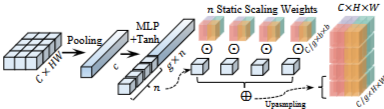
1. Pooling & Squeeze

$\begin{aligned} \text{Feature map : }&\mathbf{X} \in \mathbb{R}^{C \times H \times W}\\ \text{Global Spatial Pooling : }& z_c = \frac{1}{HW}\sum_{h,w}X_{c,h,w}\rightarrow \mathbf{z} \in \mathbb{R}^C\end{aligned}$

2. MLP + Tanh → Dynamic coefficients

• 어떤 주파수 대역을 강조해야 하는지 결정하자

$\begin{aligned} \text{MLP + Tanh - }\alpha :\ & \mathbb{R}^C \rightarrow \mathbb{R}^{g\times n} \\ \end{aligned}$

• 여기서 $\alpha$가 dynamic coefficient 이다.
  • input feature map에 따라 계속 변하는 네트워크의 예측 값이다.
  • 전체 c길이의 feature를 g개 씩 묶어서 그룹으로 만든다.

3. n Static Scaling weights

• weight matrix자체를 훈련시키기엔 너무 복잡하니까 이를 컨트롤 하는 coefficient $\alpha$와 basis $W_i$를 사용하자

$\begin{aligned}\text{static weights : } &\mathbf{W}_{\text{static weights}} \in \mathbb{R}^{\frac{C}{g} \times b \times b} \rightarrow \text{stack}\{W_1, \dots, W_n\} \in \mathbb{R}^{n \times \frac{C}{g} \times b \times b}\\ \text{final output : }& \alpha \mathbf{W}_{\text{static weights}} \in \mathbb{R}^{g \times \frac{C}{g} \times b \times b} \rightarrow \text{reshape} \in \mathbb{R}^{C\times b \times b} \end{aligned}$

• basis $W_i$는 학습을 통해 생성되고, 이를 조합하는 $\alpha$도 MLP를 통해 학습된다.

• 이렇게 학습된 basis가 각기 다른 주파수 대역으로 나뉘는 이유
  • gradient를 통해 학습되는 과정에서 각 basis가 다른 의미를 가지도록 학습하려는 경향이 있음
  • basis간 독립이 가능해야 여러 표현을 학습하기 때문임 → 이를 확인하려면, rank가 증가하는 방향으로 학습되는지 관찰하면 됨
  • 여기서 basis가 유사해 지지 않느냐? 할 수 있는데, 이를 일차적으로 방지하고자 dynamic coefficient를 제안한 것임

→ 논문에서 주장하는 내용들에 대해 코드상으로 tensor연산을 확인해 봐야 할 필요가 있음

4. Final output

$\mathbf{X} = \mathcal{F}^{-1} \left( \mathcal{F}(\mathbf{X}) \odot \mathrm{upsample}(\mathbf{W}_\text{static weights}) \right)$

• 여기서 upsampling하는 이유는 $\mathbf{W}_\text{static weights}$ 의 demension 을 $\mathcal{F}(\mathbf{X})$에 맞춰야 하기 때문이다.

3. Experiment

실험에서 확인해 보면 좋을 사항 들

• Static weight의 개수
• Dynamic coefficient의 개수
• FPS

4. Suplementary

논문에서 사용한 평가 방법 중 일부임

1. Effective Rank

$r_{\text{eff}} = \exp \left( - \sum_{i=1}^{n} \sigma_i \log \sigma_i \right)$

• 보통 rank는 0이 아닌 특이값의 개수를 말한다.
  • 여기서 일반 rank를 쓰면 0에 아주 가까운 값들 또한 유효한 값으로 취급된다.
  • 하지만, 표현 능력의 관점에서는 0에 가까운 아주 작은 수들은 제외해야 한다.
  • 이를 방지하기 위해 위 처럼 0에 가까운 값들은 무시할 수 있도록 식을 세워 사용한다.

2. Cosine Similiarity

$M_{\text{feat}}^{(l)} = \frac{2}{n(n-1)} \sum_{i=1}^{n} \sum_{j=i+1}^{n} \frac{\left|X_{i,:}^{(l)} \cdot X_{j,:}^{(l)}\right|}{\left\|X_{i,:}^{(l)}\right\|_2 \left\|X_{j,:}^{(l)}\right\|_2}$

• 단순히 i와 i-1 번째 feature 간 cos similiarity가 아니고 1번 feature와 2~n 번 feature, 2번 feature와 3~n번 feature 이런 식으로 조합 연산을 통해 계산하고 각 layer 마다 평균내는 식으로 계산한다.