Timeseries Anomaly Detection -(5) Autoencoder

Autoencoder

---

Creating an Autoencoder Model Using LSTM

import os
import tensorflow as tf
from tensorflow.keras.preprocessing.sequence import TimeseriesGenerator
from tensorflow.keras.models import Sequential
from tensorflow.keras.layers import Dense, Dropout, LSTM, RepeatVector, TimeDistributed
from tensorflow.keras.losses import Huber
from tensorflow.keras.callbacks import ModelCheckpoint, EarlyStopping
from sklearn.preprocessing import StandardScaler

# Set up random number seeds for model reproducibility
tf.random.set_seed(777)
np.random.seed(777)

# Data preprocessing - Hyperparameters
window_size = 10
batch_size = 32
features = ['Open','High','Low','Close','Volume']
n_features = len(features)
TRAIN_SIZE = int(len(df)*0.7)

# Data Preprocessing - Standard Normalization
scaler = StandardScaler()
scaler = scaler.fit(df.loc[:TRAIN_SIZE,features].values)
scaled = scaler.transform(df[features].values)

# Creating a dataset with the keras Timeseries Generator
train_gen = TimeseriesGenerator(
    data = scaled,
    targets = scaled,
    length = window_size,
    stride=1,
    sampling_rate=1,
    batch_size= batch_size,
    shuffle=False,
    start_index=0,
    end_index=None,
)

valid_gen = TimeseriesGenerator(
    data = scaled,
    targets = scaled,
    length = window_size,
    stride=1,
    sampling_rate=1,
    batch_size=batch_size,
    shuffle=False,
    start_index=TRAIN_SIZE,
    end_index=None,
)

print(train_gen[0][0].shape)  # (32, 10, 5)
print(train_gen[0][1].shape)  # (32, 5)

# Create model
# Create an encoder with two layers of LSTM
# RepeatVector copies input by window_size
model = Sequential([
    # >> encoder start
    LSTM(64, activation='relu', return_sequences=True, input_shape=(window_size, n_features)),
    LSTM(16, activation='relu', return_sequences=False),
    ## << encoder end
    ## >> Bottleneck
    RepeatVector(window_size),
    ## << Bottleneck
    ## >> decoder start
    LSTM(16, activation='relu', return_sequences=True),
    LSTM(64, activation='relu', return_sequences=False),
    Dense(n_features)
    ## << decoder end
])

# check point
# As you progress through the learning, you save the model with the best validation results
checkpoint_path = os.getenv('HOME')+'/aiffel/anomaly_detection/kospi/mymodel.ckpt'
checkpoint = ModelCheckpoint(checkpoint_path, 
                             save_weights_only=True, 
                             save_best_only=True, 
                             monitor='val_loss',
                             verbose=1)

# Early stop
# Stop when validation results get worse while learning. Patience, just watch it
early_stop = EarlyStopping(monitor='val_loss', patience=5)

model.compile(loss='mae', optimizer='adam',metrics=["mae"])

hist = model.fit(train_gen, 
          validation_data=valid_gen,
          steps_per_epoch=len(train_gen),
          validation_steps=len(valid_gen),
          epochs=50, 
          callbacks=[checkpoint, early_stop])
          

model.load_weights(checkpoint_path)
# <tensorflow.python.training.tracking.util.CheckpointLoadStatus at 0x7fa7e4312910>
fig = plt.figure(figsize=(12,8))
plt.plot(hist.history['loss'], label='Training')
plt.plot(hist.history['val_loss'], label='Validation')
plt.legend()

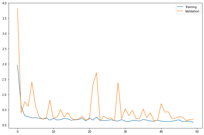
• Ensure that the training loss converges stably and the Validation loss does not diverge
• Since it is a model that predicts time series data by pushing it by window_size, the length of train_gen is shorter by window_size than the length of the original df. When comparing with the predicted result, the window_size must be skipped in front of the scaled.

# Receive prediction result as pred and performance data as real
pred = model.predict(train_gen)
real = scaled[window_size:]

mae_loss = np.mean(np.abs(pred-real), axis=1)

# Plot y-axis at log scale due to high number of samples
fig, ax = plt.subplots(figsize=(9,6))
_ = plt.hist(mae_loss, 100, density=True, alpha=0.75, log=True)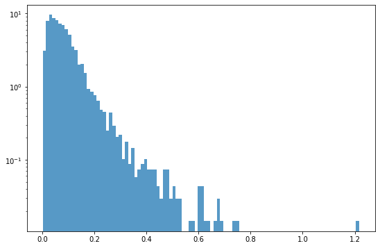

import copy

test_df = copy.deepcopy(df.loc[window_size:]).reset_index(drop=True)
test_df['Loss'] = mae_loss

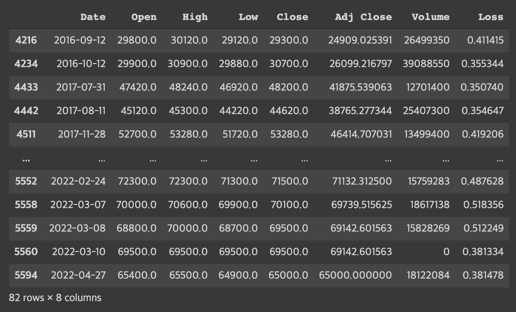
threshold = 0.35
test_df.loc[test_df.Loss>threshold]

• Looking at the point where the distribution of the Mae_loss value has decreased significantly, the corresponding values can be determined as outliers by estimating the threshold=0.35.
  

• If the threshold value is reduced to 0.3, outliers can be classified based on a stricter standard.
  • threshold=0.3

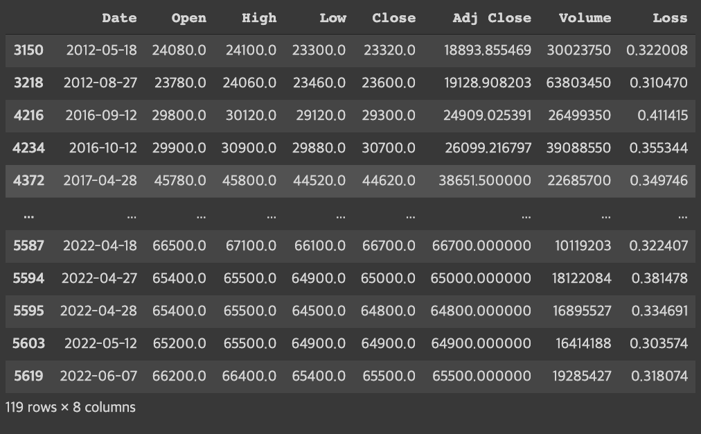
→ When the standard was stricter, 37 more outliers were found.

• Draw a graph to find outliers

fig = plt.figure(figsize=(12,15))

# graph of prices
ax = fig.add_subplot(311)
ax.set_title('Open/Close')
plt.plot(test_df.Date, test_df.Close, linewidth=0.5, alpha=0.75, label='Close')
plt.plot(test_df.Date, test_df.Open, linewidth=0.5, alpha=0.75, label='Open')
plt.plot(test_df.Date, test_df.Close, 'or', markevery=[mae_loss>threshold])

# Volume of transaction graph
ax = fig.add_subplot(312)
ax.set_title('Volume')
plt.plot(test_df.Date, test_df.Volume, linewidth=0.5, alpha=0.75, label='Volume')
plt.plot(test_df.Date, test_df.Volume, 'or', markevery=[mae_loss>threshold])

# error rate graph
ax = fig.add_subplot(313)
ax.set_title('Loss')
plt.plot(test_df.Date, test_df.Loss, linewidth=0.5, alpha=0.75, label='Loss')
plt.plot(test_df.Date, test_df.Loss, 'or', markevery=[mae_loss>threshold])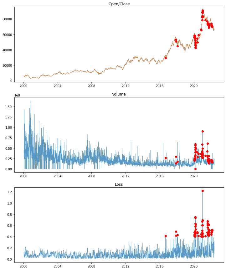

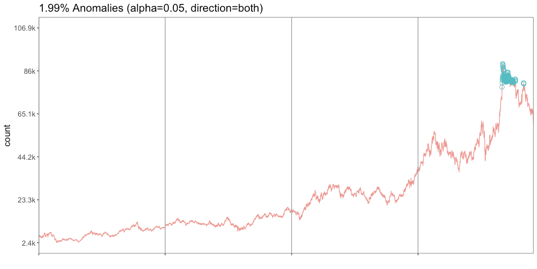
The red dot can be determined to be an outlier.

Similar results are produced when time series abnormality is detected with RStudio.