기본 통계

표준편차 = $\sqrt{\frac{\sum{|x-\mu|^2}}{N}}$
(x: 값, $\mu$: 평균, N: 모집단에 속한 자료의 개수)

avg = means(X)

def std_dev(nums, avg):
   texp = 0.0
   for i in range(len(nums)):
       texp = texp + (nums[i] - avg)**2    # 각 숫자와 평균값의 차이의 제곱을 계속 더한 후
   return (texp/(len(nums)-1)) ** 0.5    # 그 총합을 숫자개수-1로 나눈 값의 제곱근을 리턴합니다.

std_dev(X,avg)

NumPy

NumPy 주요 기능

pip install numpy

Numpy의 장점

• 빠르고 메모리를 효율적으로 사용하여 벡터의 산술 연산과 브로드캐스팅 연산을 지원하는 다차원 배열 ndarray 데이터 타입을 지원한다.
• 반복문을 작성할 필요 없이 전체 데이터 배열에 대해 빠른 연산을 제공하는 다양한 표준 수학 함수를 제공한다.
• 배열 데이터를 디스크에 쓰거나 읽을 수 있다. (즉 파일로 저장한다는 뜻입니다)
• 선형대수, 난수발생기, 푸리에 변환 가능, C/C++ 포트란으로 쓰여진 코드를 통합한다.

1) ndarray 만들기

numpy.ndarray도 array이므로 모든 element의 type이 동일해야 합니다.

A = np.arange(5)
B = np.array([0,1,2,3,4])  # 파이썬 리스트를 numpy ndarray로 변환 
C = np.array([0,1,2,3,'4'])

print(type(A))
print(type(B))
print(type(C))

>>> A와 B의 결과는 같지만 C는 모두 문자열로 바뀝니다.

2) 크기

• ndarray.size
• ndarray.shape
• ndarray.ndim
• reshape()

A = np.arange(10).reshape(2, 5)   # 길이 10의 1차원 행렬을 2X5 2차원 행렬로 바꿔봅니다.

print("행렬의 모양:", A.shape)
print("행렬의 축 개수:", A.ndim)
print("행렬 내 원소의 개수:", A.size)

3) type
NumPy의 원소는 꼭 동일한 데이터 type이어야 합니다.
dtype은 NumPy ndarray의 "원소"의 데이터타입을 반환합니다.
반면에 type(A)을 이용하면 행렬 A의 자료형이 반환됩니다.

• NumPy: numpy.array.dtype
• 파이썬: type()

A = np.arange(6).reshape(2, 3)
B = np.array([0, 1, 2, 3, 4, 5])  
C = np.array([0, 1, 2, 3, '4', 5])
D = np.array([0, 1, 2, 3, [4, 5], 6])

4) 특수행렬

• 단위행렬
• 0 행렬
• 1 행렬

np.eye(3)	# 단위행렬
np.zeros([2,3])	# 0 행렬
np.ones([3,3])	# 1행렬

5) 브로드캐스트
ndarray와 상수, 또는 서로 크기가 다른 ndarray끼리 산술연산이 가능한 기능
NumPy.org에서 제공하는 시각적인 설명자료 참고

# 차이점 구분
print([1,2]+[3,4])
print([1,2]+3)

print(np.array([1,2])+np.array([3,4]))
print(np.array([1,2])+3)

6) 슬라이스와 인덱싱
NumPy도 슬라이스와 인덱싱 연산 가능

7) random
주로 많이 쓰이는 난수

• np.random.randint()
• np.random.choice()
• np.random.permutation()
• np.random.normal()
• np.random.uniform()

print(np.random.random())   # 0에서 1사이의 실수형 난수 하나를 생성합니다. 
print(np.random.randint(0,10))   # 0~9 사이 1개 정수형 난수 하나를 생성합니다. 
print(np.random.choice([0,1,2,3,4,5,6,7,8,9]))   # 리스트에 주어진 값 중 하나를 랜덤하게 골라줍니다.

# 무작위로 섞인 배열을 만들어 줍니다. 
# 아래 2가지는 기능면에서 동일합니다. 
print(np.random.permutation(10))   
print(np.random.permutation([0,1,2,3,4,5,6,7,8,9]))

# 아래 기능들은 어떤 분포를 따르는 변수를 임의로 표본추출해 줍니다. 
# 이것은 정규분포를 따릅니다.
print(np.random.normal(loc=0, scale=1, size=5))    # 평균(loc), 표준편차(scale), 추출개수(size)
# 이것은 균등분포를 따릅니다. 
print(np.random.uniform(low=-1, high=1, size=5))  # 최소(low), 최대(high), 추출개수(size)

8) 전치행렬

• arr.T: 행렬의 행과 열 맞바꾸기
• np.transpose: 축을 기준으로 행렬의 행과 열 바꾸기

A = np.arange(24).reshape(2,3,4)
print("A:", A)               # A는 (2,3,4)의 shape를 가진 행렬입니다. 
print("A의 전치행렬:", A.T)            
print("A의 전치행렬의 shape:", A.T.shape) # A의 전치행렬은 (4,3,2)의 shape를 가진 행렬입니다.

# np.transpose는 행렬의 축을 어떻게 변환해 줄지 임의로 지정해 줄 수 있는 일반적인 행렬 전치 함수입니다. 
# np.transpose(A, (2,1,0)) 은 A.T와 정확히 같습니다.
B = np.transpose(A, (2,0,1))
print("A:", A)             # A는 (2,3,4)의 shape를 가진 행렬입니다. 
print("B:", B)             # B는 A의 3, 1, 2번째 축을 자신의 1, 2, 3번째 축으로 가진 행렬입니다.
print("B.shape:", B.shape)  # B는 (4,2,3)의 shape를 가진 행렬입니다.

NumPy로 기본 통계 데이터 계산

import numpy as np

def numbers():
    X = []
    number = input("Enter a number (<Enter key> to quit)") 
    
    while number != "":
        try:
            x = float(number)
            X.append(x)
        except ValueError:
            print('>>> NOT a number! Ignored..')
        number = input("Enter a number (<Enter key> to quit)")
    return X

def main():
    nums = numbers()       # 파이썬 리스트입니다. 
    num = np.array(nums)   # 리스트를 Numpy ndarray로 변환합니다.
    print("합", num.sum())
    print("평균값",num.mean())
    print("표준편차",num.std())
    print("중앙값",np.median(num))   # num.median() 과 혼동 조심!

main()

데이터의 행렬 변환

NumPy를 이용해 다양한 데이터 표현하는 방법을 정리한 블로그

• A Visual Intro to NumPy and Data Representation

자연어 표현 방법
임베딩(Embedding)이라는 과정을 거쳐 ndarray로 표현될 수 있다. 블로그의 예시에서는 71,290개의 단어가 들어있는 (문장들로 이루어진) 데이터셋이 있을때, 이를 단어별로 나누고 0 - 71,289로 넘버링했다. 이를 토큰화 과정이라고 한다. 이 토큰을 50차원의 word2vec embedding 을 통해 [batch_size, sequence_length, embedding_size]의 ndarray로 표현할 수 있다.

이미지의 행렬 변환

1. 픽셀과 이미지

픽셀별 명도(grayscale) 범위: 0~255 (0: 검정, 255: 흰색)

• 각각의 픽셀은 R, G, B 값 3개 요소의 튜플로 색상이 표시됩니다. (Red, Green, Blue)
  • 흰색(W) : (255,255,255)
  • 검정색(B) : (0, 0, 0)
  • 빨간색(R) : (255, 0, 0)
  • 파란색(B) : (0, 0, 255)
  • 녹색(G) : (0, 128, 0)
  • 노란색(Y) : (255, 255, 0)
  • 보라색(P) : (128, 0, 128)
  • 회색(Gray) : (128, 128, 128)
• 흑백의 경우에는 Gray 스케일로 나타내는데, 0~255 범위의 숫자 1개의 튜플 값입니다.
• Color는 투명도를 포함하는 A(alpha)를 포함해 RGBA 4개로 표시하기도 합니다.
• Image의 좌표는 보통 왼쪽 위를 (0, 0)으로 표시하고, 오른쪽과 아래로 내려갈수록 좌표가 증가합니다.

2. 이미지와 관련된 파이썬 라이브러리

• matplotlib
• PIL

import matplotlib as mpl
import PIL
print( f'# matplotlib: {mpl.__version__}' )  
print(f'# PIL:  {PIL.__version__}')

3. 간단한 이미지 조작

• open : Image.open()
• size : Image.size
• filename : Image.filename
• crop : Image.crop((x0, y0, xt, yt))
• resize : Image.resize((w,h))
• save : Image.save()

1) open

Pillow의 Image.open()이라는 메소드를 통해 이미지 파일을 open하였습니다. 이렇게 해서 얻어진 오브젝트 img는 PIL.JpegImagePlugin.JpegImageFile 라는 타입을 가지고 있습니다.

from PIL import Image, ImageColor
import os
img_path = os.getenv("HOME") + "/aiffel/data_represent/image/newyork.jpg"
img = Image.open(img_path)
print(img_path)
print(type(img))
img

2) size
이미지 파일의 타입과 색상 정보등을 확인할 수 있습니다.

print(img.format)
print(img.size)
print(img.mode)
W, H = img.size

3) 이미지 자르기
.crop() 메소드를 이용합니다. 인자로 튜플값을 받고, 가로 세로의 시작점과 가로, 세로의 종료점 총 4개를 입력해줍니다.
img.crop((30,30,100,100))

4) 저장
.save() 메소드를 사용하고 매개변수로 파일 이름을 넣어줍니다.

# 새로운 이미지 파일명
cropped_img_path = os.getenv("HOME") + "/gseung/cropped_img.jpg"
img.crop((30,30,100,100)).save(cropped_img_path)

5) 행렬로 변환
PIL.Image.Image 라는 랩퍼 클래스(Wrapper class)를 상속받은 타입을 가지고 있습니다. 이 클래스는 __array_interface__라는 속성이 정의되어 Pillow 라이브러리는 손쉽게 이미지를 Numpy ndarray로 변환 가능

img_arr = np.array(img)
print(type(img))
print(type(img_arr))
print(img_arr.shape)
print(img_arr.ndim)

6) 흑백모드
파일을 열때 흑백모드로 사진을 열 수도 있습니다. Image.open().convert('L')로 모드를 조정할 수 있습니다.
Pillow의 이미지 처리 옵션에 대한 상세한 정보는 아래를 참고하세요

• Pillow Modes

img_g = Image.open(img_path).convert('L')
img_g

7) get color

red = ImageColor.getcolor('RED','RGB')
reda = ImageColor.getcolor('red','RGBA')
yellow = ImageColor.getcolor('yellow','RGB')
print(red)
print(reda)
print(yellow)

• TensorFlow Data Augmentation Tutorials

구조화 데이터

Hash란 Key와 Value로 구성되어 있는 자료 구조로 두 개의 열만 갖지만 수많은 행을 가지는 구조체입니다.

해시는 다른 프로그래밍 언어에서는 매핑(mapping), 연관배열(associative array) 등으로 불리고 파이썬에서는 "딕셔너리(dictionary)" 또는 dict로 알려져 있습니다. 파이썬 딕셔너리는 중괄호{}를 이용하고 키 : 값의 형태로 각각 나타냅니다.

coin_per_treasure = {'rope':1,
        'apple':2,
        'torch': 2,
        'gold coin': 5, 
        'knife': 30,
        'arrow': 1}

treasure_box = {'rope': {'coin': 1, 'pcs': 2},
                'apple': {'coin': 2, 'pcs': 10},
                'torch': {'coin': 2, 'pcs': 6},
                'gold coin': {'coin': 5, 'pcs': 50},
                'knife': {'coin': 30, 'pcs': 1},
               	'arrow': {'coin': 1, 'pcs': 30}
               }

def display_stuff(treasure_box):
    print("Congraturation!! you got a treasure box!!")
    for treasure in treasure_box:
             print("You have {} {}pcs".format(treasure, treasure_box[treasure]['pcs']))
display_stuff(treasure_box)

def total_silver(treasure_box, coin_per_treasure):
    total_coin = 0
    for treasure in treasure_box:
        coin = coin_per_treasure[treasure] * treasure_box[treasure]['pcs']
        print("{} : {}coins/pcs * {}pcs = {} coins".format(
          treasure, coin_per_treasure[treasure], treasure_box[treasure]['pcs'], coin))
        total_coin += coin
    print('total_coin : ', total_coin)
total_silver(treasure_box, coin_per_treasure)

pandas

pip install pandas
구조화된 데이터를 효과적으로 표현하기 위해 pandas라는 파이썬 라이브러리는 Series와 DataFrame이라는 자료 구조를 제공합니다.

pandas의 특징

• NumPy기반에서 개발되어 NumPy를 사용하는 애플리케이션에서 쉽게 사용 가능
• 축의 이름에 따라 데이터를 정렬할 수 있는 자료 구조
• 다양한 방식으로 인덱싱(indexing)하여 데이터를 다룰 수 있는 기능
• 통합된 시계열 기능과 시계열 데이터와 비시계열 데이터를 함께 다룰 수 있는 통합 자료 구조
• 누락된 데이터 처리 기능
• 데이터베이스처럼 데이터를 합치고 관계 연산을 수행하는 기능

Series

1) Series
Series는 일련의 객체를 담을 수 있는 1차원 배열과 비슷한 자료 구조
따라서 배열 형태인 리스트, 튜플, 딕셔너리를 통해 만들거나 NumPy 자료형으로도 만들 수 있습니다.

import pandas as pd
ser = pd.Series(['a','b','c',3])
ser

Series의 인덱스(Index)

pandas의 Series에는 index와 value가 있습니다. 위에서 보면 index는 순서를 나타낸 숫자이고 value는 배열로 표현된 실제 데이터의 값입니다.

# Series 객체의 values를 호출하면 array형태로 반환됩니다.
ser.values
# 인덱스는 RangeIndex가 반환됩니다. 정수형 인덱스입니다.
ser.index

인덱스 설정: Series의 인자로 넣어주기

ser2 = pd.Series(['a', 'b', 'c', 3], index=['i','j','k','h'])
ser2

ser2.index = ['Jhon', 'Steve', 'Jack', 'Bob']
ser2

Series에서 인덱스는 기본적으로 정수 형태로 설정되고, 사용자가 원하면 값을 할당할 수 있습니다. 따라서 파이썬 딕셔너리 타입의 데이터를 Series 객체로 손쉽게 나타낼 수 있습니다.

Country_PhoneNumber = {'Korea': 82, 'America': 1, 'Swiss': 41, 'Italy': 39, 'Japan': 81, 'China': 86, 'Rusia': 7}
ser3 = pd.Series(Country_PhoneNumber)
ser3

딕셔너리의 키가 인덱스로 설정됩니다.

Series의 Name

Series 객체와 Series 인덱스는 모두 name 속성이 있습니다. 이 속성은 pandas의 DataFrame에서 매우 중요합니다.

ser3.name = 'Country_PhoneNumber'
ser3.index.name = 'Country_Name'
ser3

Series 객체의 name 속성을 이용해서 Series 객체의 이름을 설정하고, Series 인덱스의 name 속성을 이용해 인덱스 이름을 설정했습니다.

DataFrame

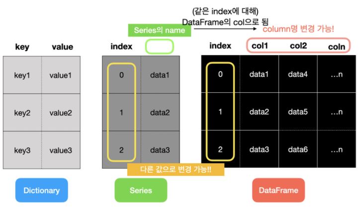
DataFrame은 표(table)와 같은 자료 구조입니다. Series는 한 개의 인덱스 컬럼과 값 컬럼, 딕셔너리는 키 컬럼과 값 컬럼과 같이 2개의 컬럼만 존재하는데 비해, DataFrame은 여러 개의 컬럼을 나타낼 수 있습니다. 그래서 csv 파일이나 excel 파일을 DataFrame으로 변환하는 경우가 많습니다.

# Series로 변환
data = {'Region' : ['Korea', 'America', 'Chaina', 'Canada', 'Italy'],
        'Sales' : [300, 200, 500, 150, 50],
        'Amount' : [90, 80, 100, 30, 10],
        'Employee' : [20, 10, 30, 5, 3]
        }
s = pd.Series(data)
s

# DataFrame으로 변환
d = pd.DataFrame(data)
d

Series는 기본적으로 인덱스 외 한 개의 값 칼럼만을 가질 수 있고 그 칼럼의 데이터가 많더라도 배열 형태로 표현됩니다.

반면 DataFrame은 인덱스 칼럼 외에도 여러 개의 칼럼을 가질 수 있습니다. 따라서 Index와 Column Index도 설정할 수 있습니다.

d.columns
d.index
d.index=['one','two','three','four','five']
d.columns = ['a','b','c','d']
d

Series의 name은 DataFrame의 Column명입니다.

실습

데이터셋 - COVID19

• covid19-italy-region.csv
  출처: 캐글 COVID-19 in Italy

CSV 파일 읽기

data = pd.read_csv(csv_path)

• head(), tail() : 처음/마지막 5개 행 출력
• .columns : 데이터셋에 존재하는 컬럼명
• .info() : 각 컬럼별로 Null값과 자료형을 보여주는 메소드
• .describe()
  : 각 컬럼별 통계 데이터(평균, 표준편차 등)를 확인. 개수(Count), 평균(mean), 표준편차(std), 최솟값(min), 4분위수(25%, 50%, 75%), 최댓값(max)를 출력
• .isnull().sum() : 결측값(Missing value) 확인 및 총합 구하기
• .value_counts()
  : 범주형 데이터로 기재되는 컬럼에 대해서는 위 메소드를 사용해 각 범주(Case 또는 Category)별로 값이 몇 개 있는지 구할 수 있습니다.
  코로나 데이터에서 범주형 데이터가 사용되는 컬럼에는 Country, RegionCode, RegionName이 있습니다.
  data['RegionName'].value_counts(), data['Country'].value_counts()
• .value_counts().sum() : ()sum 메소드를 추가해서 컬럼별 통계 수치의 합을 확인
  data['RegionName'].value_counts().sum(), data['Country'].value_counts().sum()
• .sum() : 단독으로 사용해서 해당 컬럼 값의 총합 확인

print("총감염자", data['TotalPositiveCases'].sum())
print("전체 검사자수", data['TestsPerformed'].sum())
print("사망자수", data['Deaths'].sum())
print("회복자수", data['Recovered'].sum())
data.sum()	# DataFrame 전체의 각 컬럼별로 합을 구하기

.corr()
두 컬럼 내 데이터가 얼마만큼의 상관관계가 있는지 나타냄
상관관계 분석은 EDA에서 가장 중요한 단계라고 할 수 있습니다. 이 과정을 거쳐서 불필요한 컬럼을 분석에서 제외하게 됩니다.

print(data['TestsPerformed'].corr(data['TotalPositiveCases']))
print(data['TestsPerformed'].corr(data['Deaths']))
print(data['TotalPositiveCases'].corr(data['Deaths']))

data.corr()

위와 같은 분석 작업을 통해 양성 판정 건수와 사망건수를 제외한 Country, Date, SNo, HospitalizedPatients, RegionCode, Longitude, Latitude 등의 컬럼을 삭제하기로 하였습니다. 이때 drop() 메소드가 사용됩니다.

data.drop(['Latitude','Longitude','Country','Date','HospitalizedPatients',  'IntensiveCarePatients', 'TotalHospitalizedPatients','HomeConfinement','RegionCode','SNo'], axis=1, inplace=True)

data.corr()

pandas 통계 관련 메소드

• count(): NA를 제외한 수를 반환합니다.
• describe(): 요약통계를 계산합니다.
• min(), max(): 최소, 최댓값을 계산합니다.
• sum(): 합을 계산합니다.
• mean(): 평균을 계산합니다.
• median(): 중앙값을 계산합니다.
• var(): 분산을 계산합니다.
• std(): 표준편차를 계산합니다.
• argmin(), argmax(): 최소, 최댓값을 가지고 있는 값을 반환 합니다.
• idxmin(), idxmax(): 최소, 최댓값을 가지고 있는 인덱스를 반환합니다.
• cumsum(): 누적 합을 계산합니다.
• pct_change(): 퍼센트 변화율을 계산합니다.

---

Pandas 공식문서에서 정리한 Pandas 주요 기능 (소요시간 30분 ~ 1시간)

• 10 minutes to pandas