학습 목표
- 딥러닝 문제 구성에 대한 기본적인 이해를 높인다.
- Neural Network에 사용되는 용어들에 대한 이해를 높인다.
- 딥러닝 프레임워크를 사용하지 않고, Numpy만을 이용해 딥러닝 모델과 훈련 과정을 직접 구현해 본다.
퍼셉트론(Perceptron): 뇌의 신경망 구조의 착안해 만든 인공신경망의 한 종류
MNIST 이미지 분류기
Conv2D와 같이 이미지 분류에 특화된 모델이 아닌 다츷 퍼셉트론(MLP)만을 이용해 더욱 간단하게 구현이 가능합니다.
import tensorflow as tf
from tensorflow import keras
import numpy as np
import matplotlib.pyplot as plt

# MNIST 데이터를 로드. 다운로드하지 않았다면 다운로드까지 자동으로 진행됩니다.
mnist = keras.datasets.mnist
(x_train, y_train), (x_test, y_test) = mnist.load_data()

# 모델에 맞게 데이터 가공
x_train_norm, x_test_norm = x_train / 255.0, x_test / 255.0
x_train_reshaped = x_train_norm.reshape(-1, x_train_norm.shape[1]*x_train_norm.shape[2])
x_test_reshaped = x_test_norm.reshape(-1, x_test_norm.shape[1]*x_test_norm.shape[2])

# 딥러닝 모델 구성 - 2 Layer Perceptron
model=keras.models.Sequential()
model.add(keras.layers.Dense(50, activation='sigmoid', input_shape=(784,)))  # 입력층 d=784, 은닉층 레이어 H=50
model.add(keras.layers.Dense(10, activation='softmax'))   # 출력층 레이어 K=10
model.summary()

# 모델 구성과 학습
model.compile(optimizer='adam',
             loss='sparse_categorical_crossentropy',
             metrics=['accuracy'])
model.fit(x_train_reshaped, y_train, epochs=10)

# 모델 테스트 결과
test_loss, test_accuracy = model.evaluate(x_test_reshaped,y_test, verbose=2)
print("test_loss: {} ".format(test_loss))
print("test_accuracy: {}".format(test_accuracy))
다층 퍼셉트론 Overview
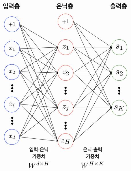
보통 2개 이상의 레이어를 쌓아서 만든 인공신경망
깊어지면 DNN(Deep Neural Network)라고 부릅니다.
참고자료 - bias term
Tips
Fully-Connected Neural Network는 MLP의 다른 용어. 서로 다른 층에 위치한 노드 간에는 연결 관계가 존재하지 않으며, 인접한 층에 위치한 노드들 간의 연결만 존재한다는 의미를 내포합니다.
Parameters/Weights
입력값이 100개, 은닉 노드가 20개라면 입력층-은닉층 사이에는 100x20의 shape을 가진 행렬이 존재합니다.
인점한 레이어 사이에는 아래와 같은 관계가 성립합니다.
위에서 만들었던 MLP기반 딥러닝 모델을 Numpy로 구현하면 아래와 같습니다.
# 입력층 데이터의 모양(shape)
print(x_train_reshaped.shape)

# 테스트를 위해 x_train_reshaped의 앞 5개의 데이터를 가져온다.
X = x_train_reshaped[:5]
print(X.shape)

weight_init_std = 0.1
input_size = 784
hidden_size=50

# 인접 레이어간 관계를 나타내는 파라미터 W를 생성하고 random 초기화
W1 = weight_init_std * np.random.randn(input_size, hidden_size)
# 바이어스 파라미터 b를 생성하고 Zero로 초기화
b1 = np.zeros(hidden_size)

a1 = np.dot(X, W1) + b1   # 은닉층 출력

print(W1.shape)
print(b1.shape)
print(a1.shape)

# 첫 번째 데이터의 은닉층 출력을 확인해 봅시다.  50dim의 벡터가 나오나요?
a1[0]
활성함수와 손실함수
활성화 함수(Activation Function)
활성화 함수로 비선형 함수를 추가함으로써 비선형성을 더해줍니다.
1. Sigmoid
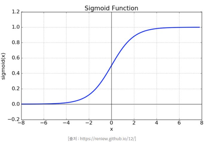
사용 예시
model.add(keras.layers.Dense(50, activation='sigmoid', input_shape=(784,)))
문제점
- Vanishing gradient 현상이 발생한다.
- exp 함수 사용 시 비용이 크다.
2. Tanh
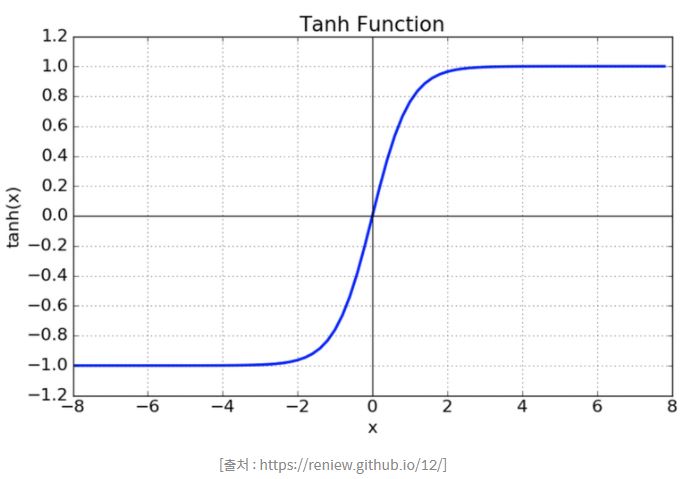
- tanh 함수는 한수의 중심값을 0으로 옮겨 sigmoid의 최적화 과정이 느려지는 문제를 해결
- 여전히 Vanishing gradient 문제 존재
3. ReLU
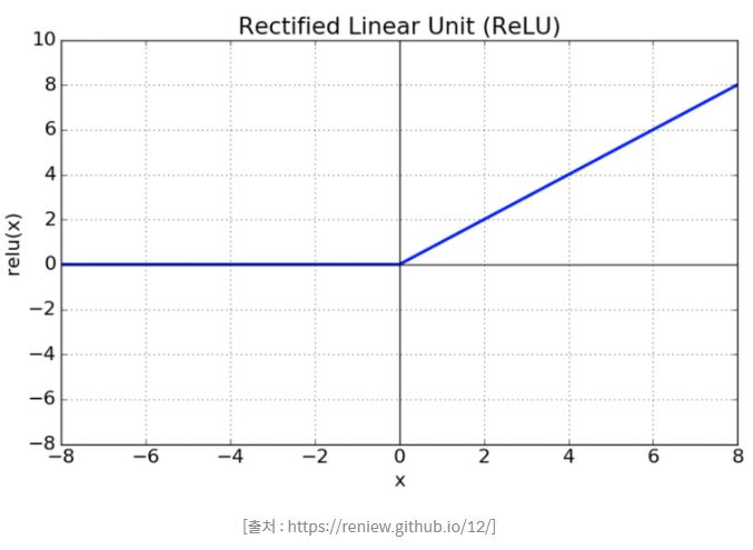
- sigmoid, tanh 함수에 비해 학습이 빠름
- 연산 비용이 크지 않고, 구현이 매우 간단하다.
MLP Layer 구현
# 단일 레이어 구현 함수
def affine_layer_forward(X, W, b):
    y = np.dot(X, W) + b
    cache = (X, W, b)
    return y, cache

input_size = 784
hidden_size = 50
output_size = 10

W1 = weight_init_std * np.random.randn(input_size, hidden_size)
b1 = np.zeros(hidden_size)
W2 = weight_init_std * np.random.randn(hidden_size, output_size)
b2 = np.zeros(output_size)

a1, cache1 = affine_layer_forward(X, W1, b1)
z1 = sigmoid(a1)
a2, cache2 = affine_layer_forward(z1, W2, b2)    # z1이 다시 두번째 레이어의 입력이 됩니다.

print(a2[0])  # 최종 출력이 output_size만큼의 벡터가 되었습니다.

def softmax(x):
    if x.ndim == 2:
        x = x.T
        x = x - np.max(x, axis=0)
        y = np.exp(x) / np.sum(np.exp(x), axis=0)
        return y.T

    x = x - np.max(x) # 오버플로 대책
    return np.exp(x) / np.sum(np.exp(x))

y_hat = softmax(a2)
y_hat[0]  # 10개의 숫자 중 하나일 확률이 되었습니다.
손실함수(Loss Function)
평균제곱오차 (MSE:Mean Square Error)
교차 엔트로피(Cross Entropy)
두 확률분포 사이의 유사도가 클수록 작아지는 값입니다.
경사하강법
각 시점의 기울기가 가리키는 방향으로 이동하는 것입니다.
학습률(learning rate)이라는 개념을 도입해 기울기 값과 이 학습률을 곱한 만큼만 발걸음을 내딛습니다.
하지만 어디서 출발했느냐에 따라 산 아래로 내려가는 시간이 빨라질 수도 느려질 수도 있습니다. 이는 parameter의 값들을 어떻게 초기화하는지의 문제와 맞닿아 있습니다.
참고 자료
- [ ML ] 모두를 위한 TensorFlow (3) Gradient descent algorithm 기본
- 가중치 초기화 (Weight Initialization)
- [머신러닝] lec 7-1 : 학습 Learning rate, Overfitting, 그리고 일반화
batch_num = y_hat.shape[0]
dy = (y_hat - t) / batch_num
dy
위에서
dy가 구해지면 다른 기울기들은 chain-rule로 쉽게 구할 수 있습니다.
같은 방식으로 학습해야 할 모든 파라미터 W1, b1, W2, b2에 대한 기울기를 모두 얻을 수 있습니다.
dW2 = np.dot(z1.T, dy)
db2 = np.sum(dy, axis=0)
# 중간에 sigmoid가 한번 사용되었으므로, 활성화함수에 대한 gradient도 고려되어야 합니다.
def sigmoid_grad(x):
return (1.0 - sigmoid(x)) * sigmoid(x)
dz1 = np.dot(dy, W2.T)
da1 = sigmoid_grad(a1) * dz1
dW1 = np.dot(X.T, da1)
db1 = np.sum(dz1, axis=0)
# 파라미터를 업데이트 하는 경우
learning_rate = 0.1
def update_params(W1, b1, W2, b2, dW1, db1, dW2, db2, learning_rate):
W1 = W1 - learning_rate*W1
b1 = b1 - learning_rate*db1
W2 = W2 - learning_rate*dW2
b2 = b2 - learning_rate*db2
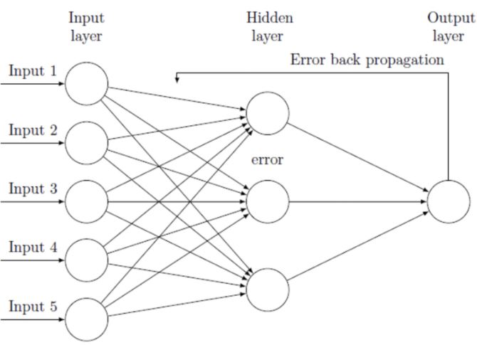
return W1, b1, W2, b2오차역전파법이란?
오차역전파법(Backpropagation)이란 학습시킬 때 사용하는 알고리즘 중 하나입니다. 이는 출력층의 결과와 내가 뽑고자 하는 target 값과의 차이를 구한 뒤, 그 오차 값을 각 레이어들을 지나며 역전파 해가며 각 노드가 가지고 있는 변수들을 갱신해 나가는 방식입니다.
이전의 affine_layer_forward(X, W, b)에 대응하여 해당 레이어의 backpropagation 함수를 얻을 수 있습니다.
def affine_layer_backward(dy, cache):
    X, W, b = cache
    dX = np.dot(dy, W.T)
    dW = np.dot(X.T, dy)
    db = np.sum(dy, axis=0)
    return dX, dW, db
지금까지 내용을 바탕으로 Forward Propagation과 Backward Propagation이 이루어지는 단계는 아래와 같습니다.
모델 학습 Step-by-Step
# 파라미터 초기화
W1 = weight_init_std * np.random.randn(input_size, hidden_size)
b1 = np.zeros(hidden_size)
W2 = weight_init_std * np.random.randn(hidden_size, output_size)
b2 = np.zeros(output_size)

def train_step(X, Y, W1, b1, W2, b2, learning_rate=0.1, verbose=False):
    # Forward Propagation
    a1, cache1 = affine_layer_forward(X, W1, b1)
    z1 = sigmoid(a1)
    a2, cache2 = affine_layer_forward(z1, W2, b2)

    # 추론과 오차(Loss) 계산
    y_hat = softmax(a2)
    t = _change_one_hot_label(Y_digit, 10)   # 정답 One-hot 인코딩
    Loss = cross_entropy_error(y_hat, t)

    if verbose:
        print('---------')
        print(y_hat)
        print(t)
        print('Loss: ', Loss)

    dy = (y_hat - t) / X.shape[0]
    dz1, dW2, db2 = affine_layer_backward(dy, cache2)
    da1 = sigmoid_grad(a1) * dz1
    dX, dW1, db1 = affine_layer_backward(da1, cache1)

    # 경사하강법을 통한 파라미터 업데이트
    W1, b1, W2, b2 = update_params(W1, b1, W2, b2, dW1, db1, dW2, db2, learning_rate)

    return W1, b1, W2, b2, Loss


X = x_train_reshaped[:5]
Y = y_train[:5]

# train_step을 다섯 번 반복 돌립니다.
for i in range(5):
    W1, b1, W2, b2, _ = train_step(X, Y, W1, b1, W2, b2, learning_rate=0.1, verbose=True)
추론 과정 구현과 정확도(Accuracy) 계산
위에서 5번 학습한 파라미터 W1, b1, W2, b2를 가지고 숫자를 인식(Predict)하고 그 정확도(Accuracy)를 측정할 수 있습니다.
def predict(W1, b1, W2, b2, X):
    a1 = np.dot(X, W1) + b1
    z1 = sigmoid(a1)
    a2 = np.dot(z1, W2) + b2
    y = softmax(a2)

    return y

# X = x_train[:100] 에 대해 모델 추론을 시도합니다.
X = x_train_reshaped[:100]
Y = y_test[:100]
result = predict(W1, b1, W2, b2, X)
result[0]

def accuracy(W1, b1, W2, b2, x, y):
    y_hat = predict(W1, b1, W2, b2, x)
    y_hat = np.argmax(y_hat, axis=1)

    accuracy = np.sum(y_hat == y) / float(x.shape[0])
    return accuracy


acc = accuracy(W1, b1, W2, b2, X, Y)

t = _change_one_hot_label(Y, 10)
print(result[0])
print(t[0])
print(acc)
하지만 학습의 반복(iteration)이 적어 10% 이하의 정확도를 가지므로 전체 학습 사이클을 수행합니다.
전체 학습 사이클 수행
def init_params(input_size, hidden_size, output_size, weight_init_std=0.01):

    W1 = weight_init_std * np.random.randn(input_size, hidden_size)
    b1 = np.zeros(hidden_size)
    W2 = weight_init_std * np.random.randn(hidden_size, output_size)
    b2 = np.zeros(output_size)

    print(W1.shape)
    print(b1.shape)
    print(W2.shape)
    print(b2.shape)

    return W1, b1, W2, b2

# 하이퍼파라미터
iters_num = 50000  # 반복 횟수를 적절히 설정한다.
train_size = x_train.shape[0]
batch_size = 100   # 미니배치 크기
learning_rate = 0.1

train_loss_list = []
train_acc_list = []
test_acc_list = []

# 1에폭당 반복 수
iter_per_epoch = max(train_size / batch_size, 1)

W1, b1, W2, b2 = init_params(784, 50, 10)

for i in range(iters_num):
    # 미니배치 획득
    batch_mask = np.random.choice(train_size, batch_size)
    x_batch = x_train_reshaped[batch_mask]
    y_batch = y_train[batch_mask]

    W1, b1, W2, b2, Loss = train_step(x_batch, y_batch, W1, b1, W2, b2, learning_rate=0.1, verbose=False)

    # 학습 경과 기록
    train_loss_list.append(Loss)

    # 1에폭당 정확도 계산
    if i % iter_per_epoch == 0:
        print('Loss: ', Loss)
        train_acc = accuracy(W1, b1, W2, b2, x_train_reshaped, y_train)
        test_acc = accuracy(W1, b1, W2, b2, x_test_reshaped, y_test)
        train_acc_list.append(train_acc)
        test_acc_list.append(test_acc)
        print("train acc, test acc | " + str(train_acc) + ", " + str(test_acc))
이렇게 딥러닝 프레임워크 없이 Numpy만으로 딥러닝이 가능합니다.
위 훈련 과정의 Accuracy, Loss 변화를 시각화합니다.
from matplotlib.pylab import rcParams
rcParams['figure.figsize'] = 12, 6

# Accuracy 그래프 그리기
markers = {'train': 'o', 'test': 's'}
x = np.arange(len(train_acc_list))
plt.plot(x, train_acc_list, label='train acc')
plt.plot(x, test_acc_list, label='test acc', linestyle='--')
plt.xlabel("epochs")
plt.ylabel("accuracy")
plt.ylim(0, 1.0)
plt.legend(loc='lower right')
plt.show()

# Loss 그래프 그리기
x = np.arange(len(train_loss_list))
plt.plot(x, train_loss_list, label='train acc')
plt.xlabel("epochs")
plt.ylabel("Loss")
plt.ylim(0, 3.0)
plt.legend(loc='best')
plt.show()
Reference