텍스트### 1. Markov chain monte carlo(MCMC)
- Construct a markov chain whose stationary distribution = to draw samples from target distribution .
- Running a markov chain leads to sampling from target distribution
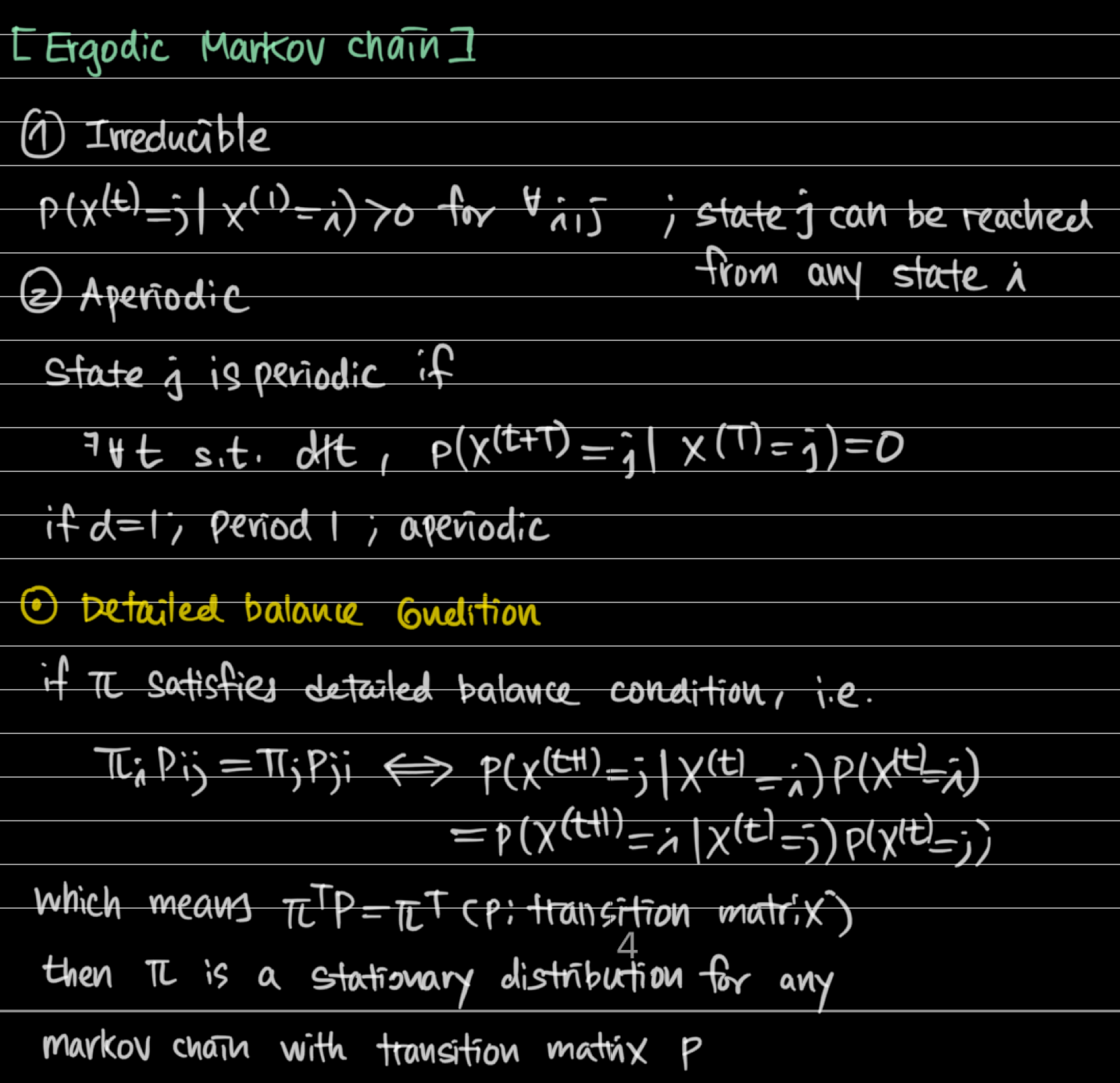
- Ergoic markov chain has unique stationary distribution
- Bayesian inference can be done on markov chain samples, even when the posterior distribution is intractable.
- Definition of markov chain:
- Transition probability: , time homogeneous condition: is constant
- is a stationary distribution if
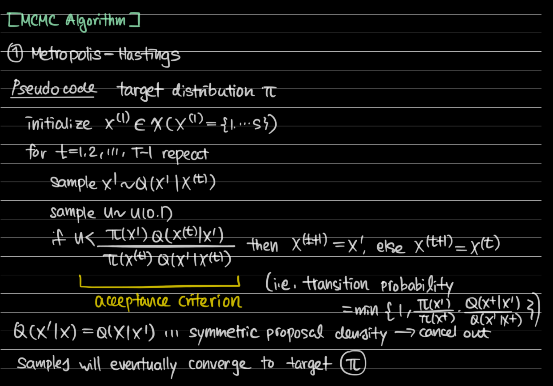
2. Metropolis-Hastings algorithm
- Metropolis-Hastings algorithm can be utilized even if we only know the kernel of the target distribution.
- Acceptance criterion is designed to meet the detailed balance condition
- Symmetric proposal density, extremely we can utilize uniform distribution of Bernoulli(0.5) for some special variables. Usually normal proposal density is utilized(random walk metropolis samples with a symmetric normal proposal).
- Practical issues
- Burn-in(discard first several samples to remove the effect caused by the arbitrary starting point)
- Thinning(only select Mth sample to obtain independent samples)
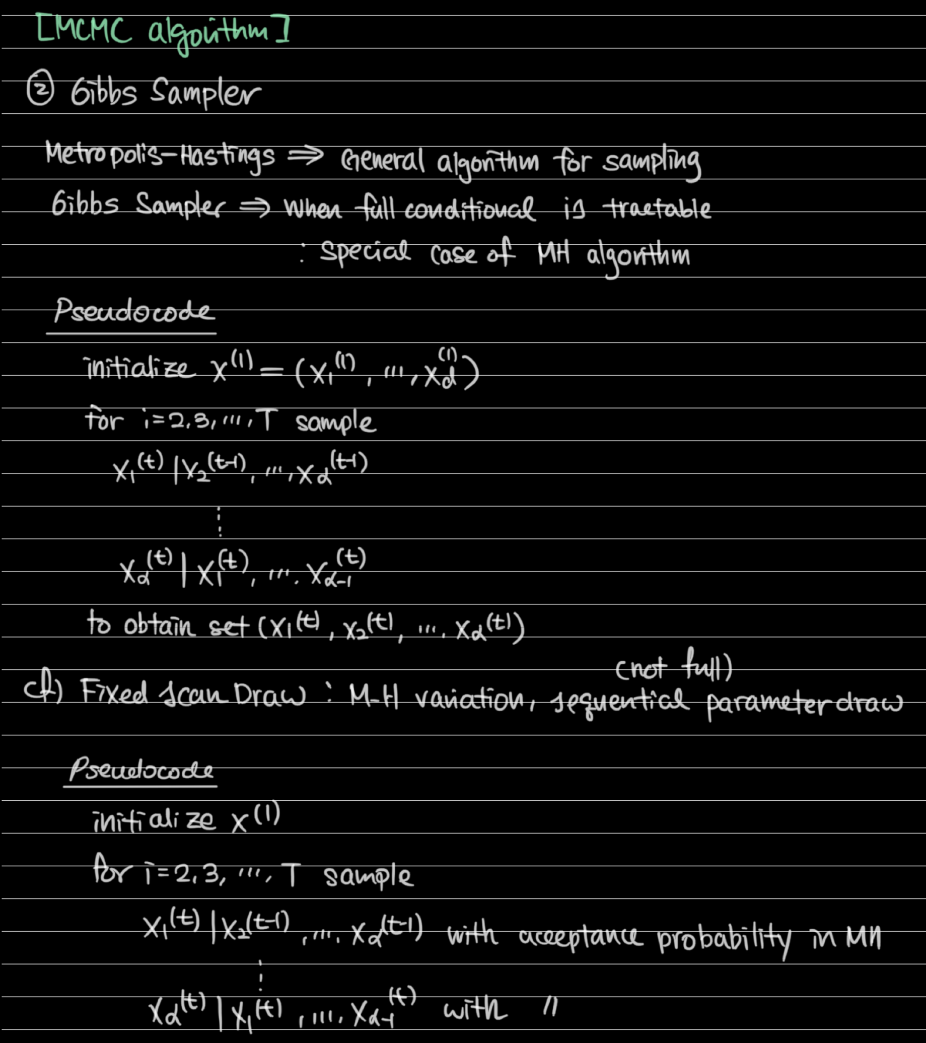
3. Gibbs Sampler
- Gibbs Sampler can be utilized when we know the full conditional distribution of target distribution.
- Fixed-scan draw is similar to gibbs sampler, while Metropolis-Hastings style acceptance criterion is added for each sequential parameter draw process.
4. Diagnostic methods and Practical issues
- Burn-in, Thinning
- Metropolis-hastings algorithm: random walk sampler, step size also should be tuned
- Step size can be tuned separately for multivariate cases, but step size also can be tuned adaptively
- where is a sample covariance matrix using posterior samples up to nth iteration
- Adaptive updates should be stopped in some N< iteration
- To remove intial value effect, you can utilize burn-in or try MLE estimate as an intial value, or try different initial values and run chains separately
[Diagnostic Methods]
- TS plot
- Density plot
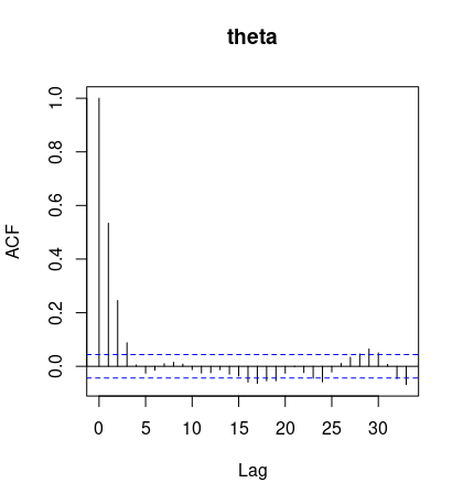
- Autocrrelation function(ACF plot)
- Effective sample size
- Gelman-rubin statistic(ANOVA test-like statistic)
- Remark: If autocorrelation remains high, we should consider thinning to increase effective sample size... Figure below is fine.

interested in 🖥️,🧠,🧬,⚛️