[MLOps] MLflow 시작하기

MLflow

MLflow
MLflow는 Databricks에서 개발한 머신러닝 워크플로우를 관리하고 간소화하기 위한 오픈소스 플랫폼입니다.
ML 모델의 개발, 추적, 배포, 관리 등 전체 수명 주기를 지원합니다.

구성 요소

1. MLflow Tracking

• 실험 데이터를 추적하고 기록하며, 파라미터, 메트릭, 코드 버전, 아티팩트를 저장합니다.
• UI를 통해 실험 결과를 시각화하고 비교할 수 있습니다.

  아티팩트(Artifact)
  실험이나 모델 훈련 과정에서 생성되는 출력물
  모델, 데이터 파일, 체크포인트, 로그, 메타데이터 등 다양한 형태

2. MLflow Projects

• 재사용 가능하도록 ML 코드를 패키징합니다.
• 여러 프로젝트를 체인화해 다단계 워크플로우 생성이 가능합니다.
• 프로젝트는 코드와 의존성을 포함하는 디렉토리 또는 Git 저장소입니다.
• MLproject 파일은 프로젝트의 메타데이터를 정의하는 YAML 형식의 파일입니다. 즉, MLproject 파일은 프로젝트의 실행 방법과 환경을 정의하는 설정 파일입니다.

3. MLflow Models

• 다양한 ML 라이브러리에서 생성된 모델을 패키징하고 배포할 수 있습니다.
• 모델은 여러 Flavor로 저장됩니다. (예시: sklearn, tensorflow, pytorch)

4. MLflow Model Registry

• 모델의 전체 수명 주기를 관리하는 중앙 저장소를 제공합니다.
• 모델 버전 관리, 상태 전환, 주석 추가 및 모델 계보 추적이 가능합니다.

MLflow 튜토리얼 진행하기

작업할 디렉토리를 하나 생성하겠습니다.

mkdir mlflow-tutorial
cd mlflow-tutorial

가상환경을 하나 생성해줍니다.

python -m venv venv
source venv/bin/activate 

필요한 라이브러리들을 설치합니다.

pip install mlflow scikit-learn pandas matplotlib seaborn

기본 ML 학습 코드

Iris 데이터셋의 Classification 코드를 작성합니다.

# basic.py
from sklearn.datasets import load_iris
from sklearn.ensemble import RandomForestClassifier
from sklearn.metrics import accuracy_score
from sklearn.model_selection import train_test_split

# 1. 데이터 로딩
iris = load_iris()
X_train, X_test, y_train, y_test = train_test_split(
    iris.data, iris.target, test_size=0.2, random_state=42
)

# 2. 모델 정의 및 학습
n_estimators = 100
max_depth = 3

model = RandomForestClassifier(n_estimators=n_estimators, max_depth=max_depth, random_state=42)
model.fit(X_train, y_train)

# 3. 예측 및 정확도 평가
preds = model.predict(X_test)
accuracy = accuracy_score(y_test, preds)

print(f"Accuracy: {accuracy:.4f}")

결과

Accuracy: 1.0000

MLflow 적용 학습 코드

이번엔 MLflow를 적용한 tutorial.py를 작성합니다.

# tutorial.py
import mlflow
import mlflow.sklearn
import pandas as pd
import matplotlib.pyplot as plt
import seaborn as sns
import os
from sklearn.datasets import load_iris
from sklearn.ensemble import RandomForestClassifier
from sklearn.metrics import accuracy_score, confusion_matrix
from sklearn.model_selection import train_test_split

# 1. 실험 이름 지정
mlflow.set_experiment("MLFlow_Tutorial")

# 데이터 로딩
iris = load_iris()
X_train, X_test, y_train, y_test = train_test_split(
    iris.data, iris.target, test_size=0.2, random_state=42
)

# 2. 실험 시작
with mlflow.start_run(run_name="RF_100_3"):
    # 하이퍼파라미터
    n_estimators = 100
    max_depth = 3

    # 모델 학습
    model = RandomForestClassifier(n_estimators=n_estimators, max_depth=max_depth, random_state=42)
    model.fit(X_train, y_train)

    # 예측 및 평가
    preds = model.predict(X_test)
    accuracy = accuracy_score(y_test, preds)

    # 3. 메트릭 및 파라미터 로깅
    mlflow.log_param("n_estimators", n_estimators)
    mlflow.log_param("max_depth", max_depth)
    mlflow.log_metric("accuracy",  accuracy)

    # 4. 모델 아티팩트 저장
    mlflow.sklearn.log_model(model, "iris_rf_model")

    cm = confusion_matrix(y_test, preds)
    plt.figure(figsize=(6, 4))
    sns.heatmap(cm, annot=True, fmt="d", cmap="Blues", xticklabels=iris.target_names, yticklabels=iris.target_names)
    plt.title("Confusion Matrix")
    plt.xlabel("Predicted")
    plt.ylabel("True")
    plt.tight_layout()

    # 5. 파일로 저장 후 artifact로 로깅
    os.makedirs("outputs", exist_ok=True)
    fig_path = "outputs/conf_matrix.png"
    plt.savefig(fig_path)
    mlflow.log_artifact(fig_path)

    # 6. 태그 설정
    mlflow.set_tag("model_type", "RandomForest")
    mlflow.set_tag("version", "v1.0")
    mlflow.set_tag("developer", "hanseul37")

    print(f"Accuracy: {accuracy:.4f}")

1. 실험 이름 지정

mlflow.set_experiment("MLFlow_Tutorial")

• MLflow에서 실험 이름을 설정합니다. 실험은 여러 실행을 그룹화하는 역할을 합니다.
• 지정된 이름(MLFlow_Tutorial)의 실험이 존재하지 않으면 새로 생성됩니다.
• 모든 실행은 이 실험에 속하게 됩니다.

2. 실험 시작

with mlflow.start_run(run_name="RF_100_3"):

• 새로운 실행을 시작합니다. run_name은 실행의 이름으로 지정됩니다.
• 실행은 모델 학습, 평가, 로깅 등의 작업을 포함하며, MLflow UI에서 개별 실행을 확인할 수 있습니다.
  

3. 메트릭 및 파라미터 로깅

mlflow.log_param("n_estimators", n_estimators)
mlflow.log_param("max_depth", max_depth)
mlflow.log_metric("accuracy",  accuracy)

• 모델 설정에 사용된 값인 하이퍼파라미터를 로깅합니다.
• 모델 성능을 나타내는 값인 메트릭을 로깅합니다.

4. 모델 아티팩트 저장

mlflow.sklearn.log_model(model, "iris_rf_model")

• 학습된 모델을 저장하고 MLflow에 로깅합니다.
• 저장된 모델은 MLflow UI나 API를 통해 다시 불러올 수 있습니다.
• iris_rf_model은 모델의 이름으로 지정됩니다.

5. 파일로 저장 후 아티팩트 로깅

mlflow.log_artifact(fig_path)

• 생성된 파일을 MLflow에 로깅합니다. 이 파일은 MLflow UI에서 확인하거나 다운로드할 수 있습니다.

6. 태그 설정

mlflow.set_tag("model_type", "RandomForest")
mlflow.set_tag("version", "v1.0")
mlflow.set_tag("developer", "hanseul37")

• 태그는 실행에 추가적인 정보를 제공하는 메타데이터입니다.
  • model_type: 사용한 모델 유형
  • version: 현재 실행의 버전 정보
  • developer: 개발자 이름

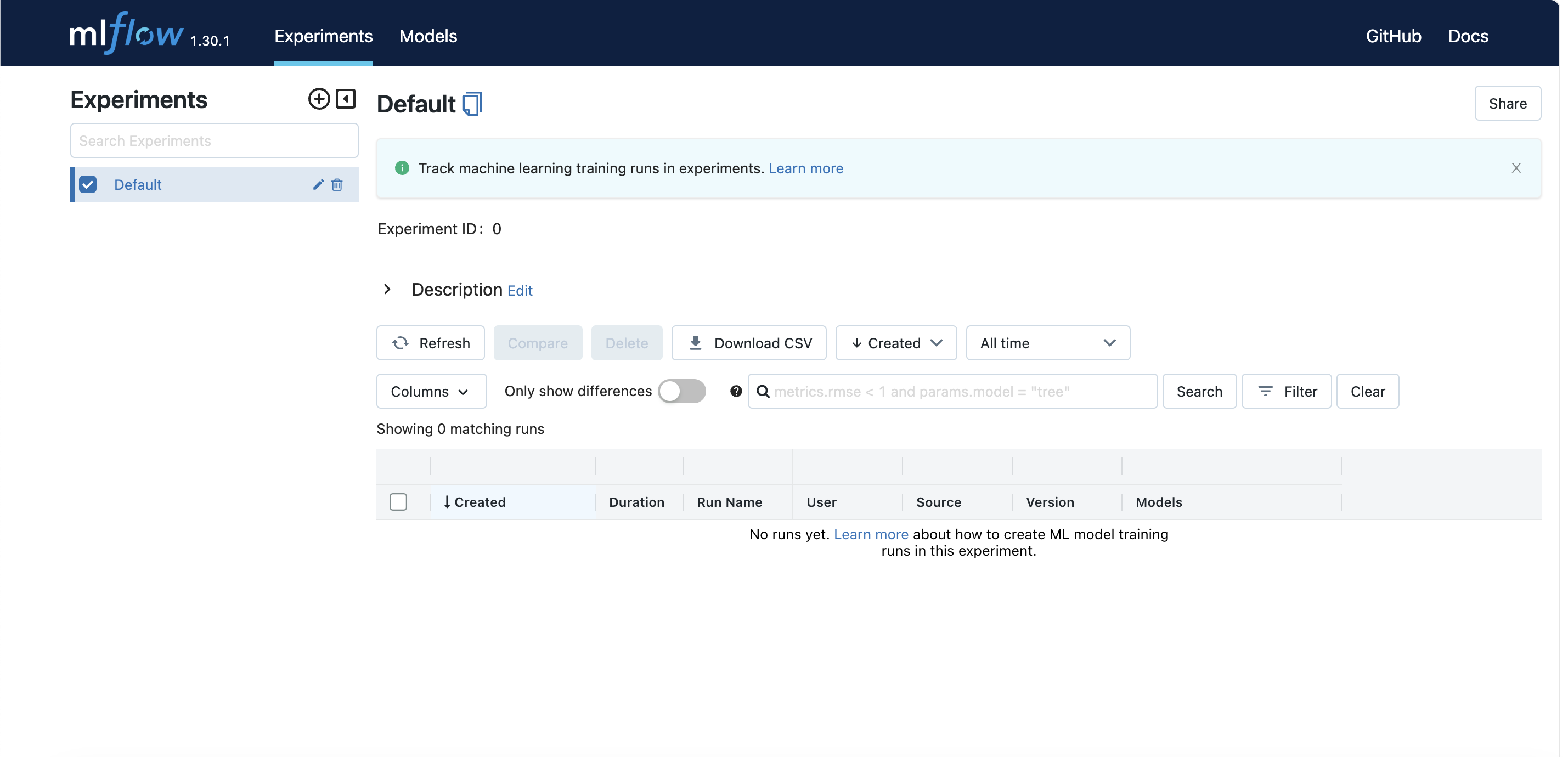
mlflow UI 서버를 실행합니다.

mlflow ui

http://localhost:5000 으로 접속하면 아래처럼 UI에 접속할 수 있습니다.

이제 tutorial.py를 실행해보면 UI에서 생성한 실험을 확인할 수 있습니다.

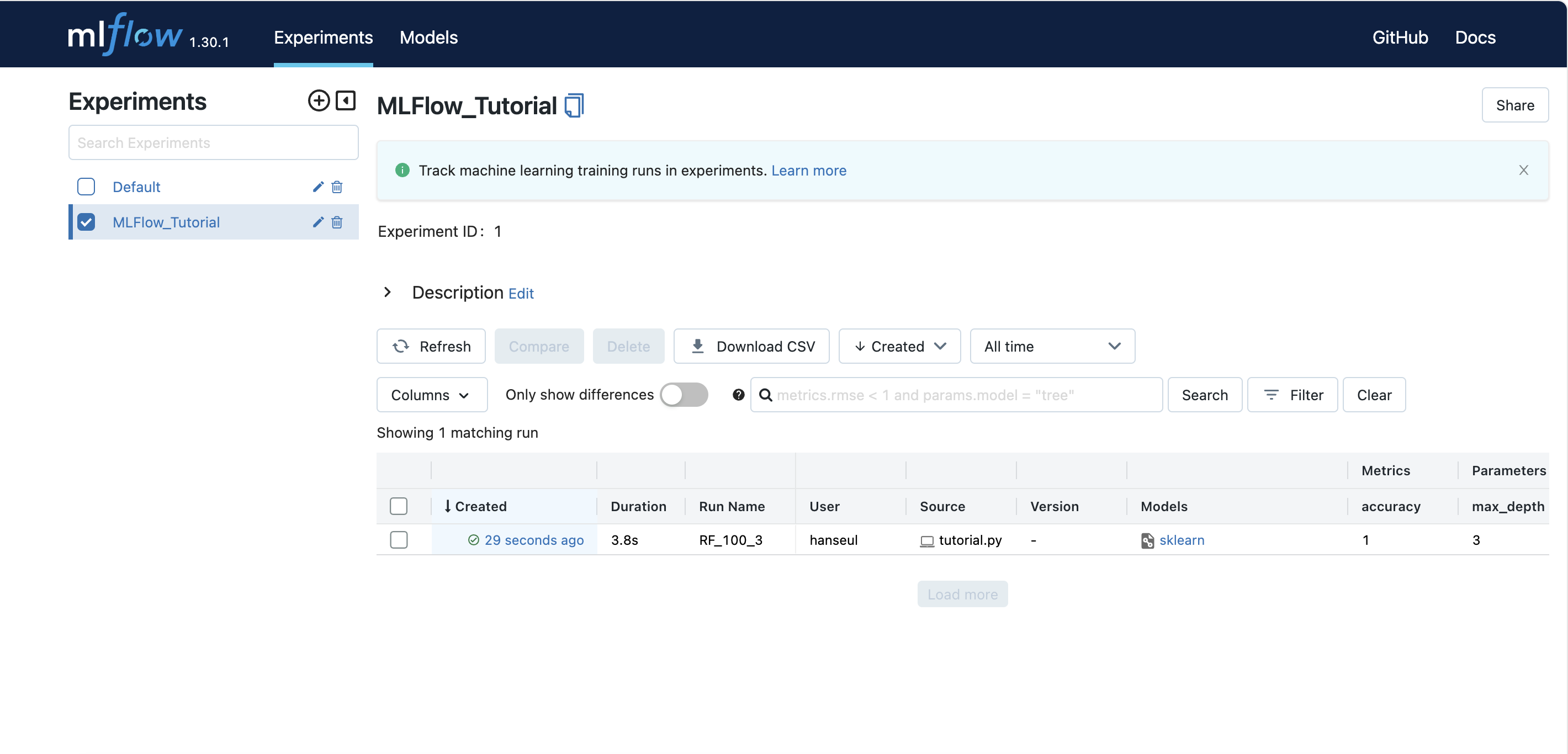
실험 진행 시간, Run 이름, 메트릭, 파라미터, 태그 정보를 확인할 수 있습니다.

파란색 글씨를 클릭하면 실행 세부 정보로 들어갈 수 있습니다.

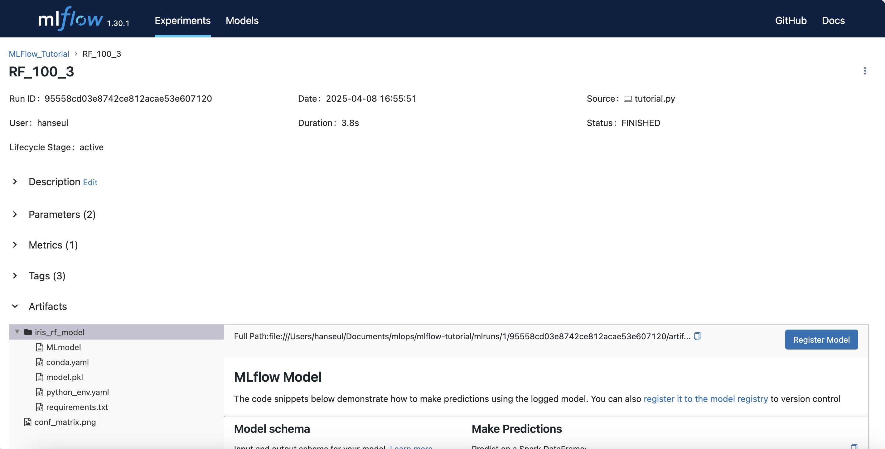
이 곳에서도 파라미터, 메트릭, 태그 정보들을 확인할 수 있습니다.

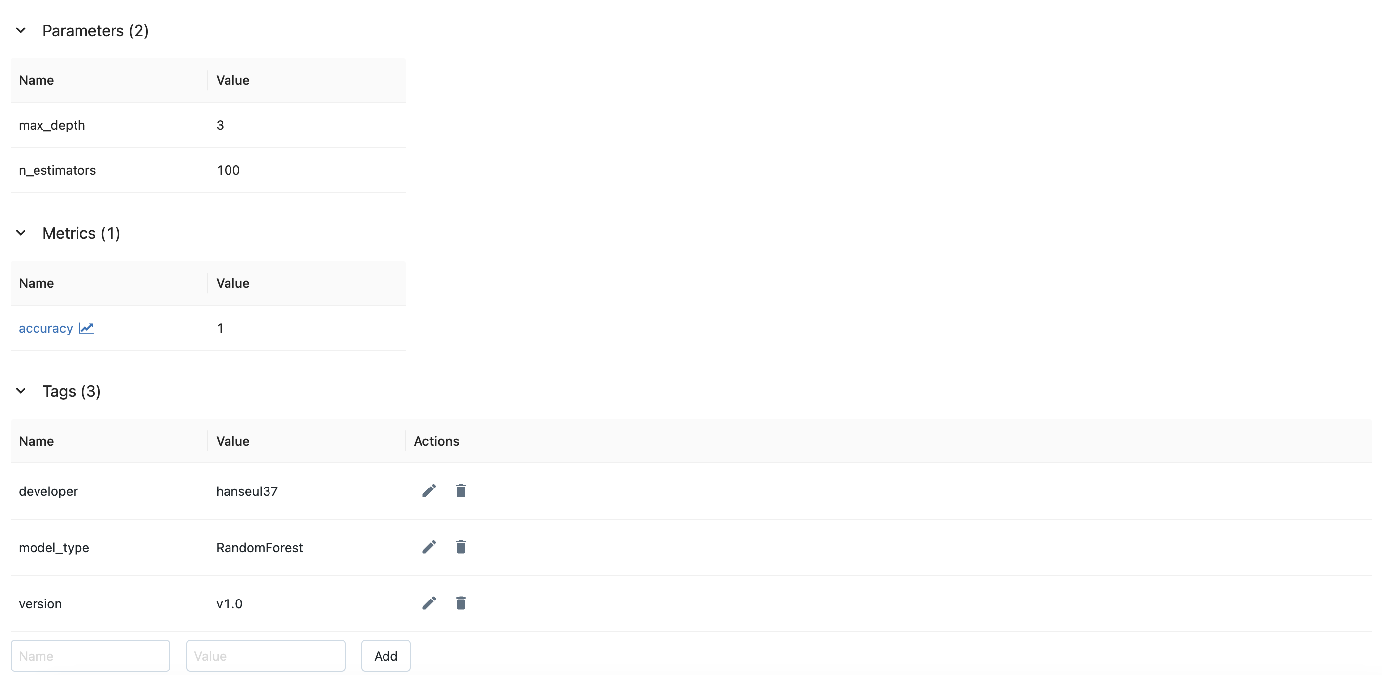
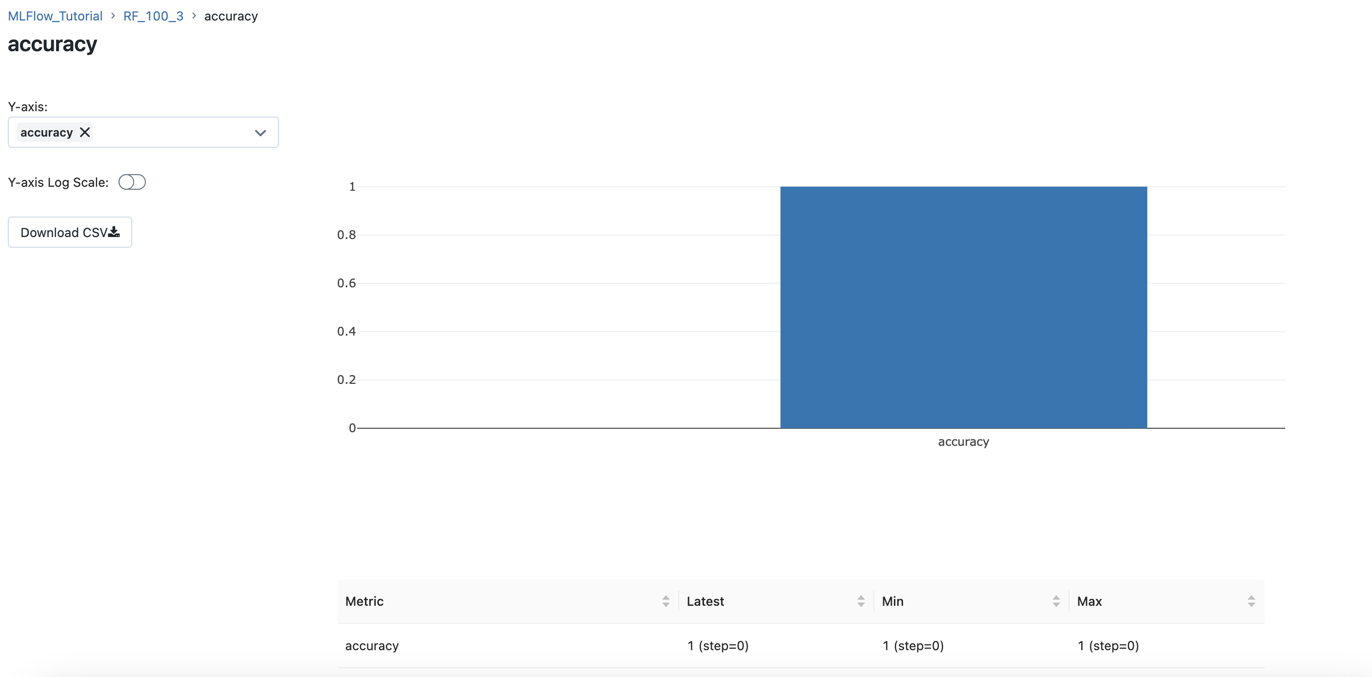
메트릭을 클릭하면, 메트릭의 세부 그래프를 확인할 수 있습니다.

아티팩트를 확인하면, 코드에서 저장한 혼동 행렬이 저장되어 있는 것을 확인할 수 있습니다.

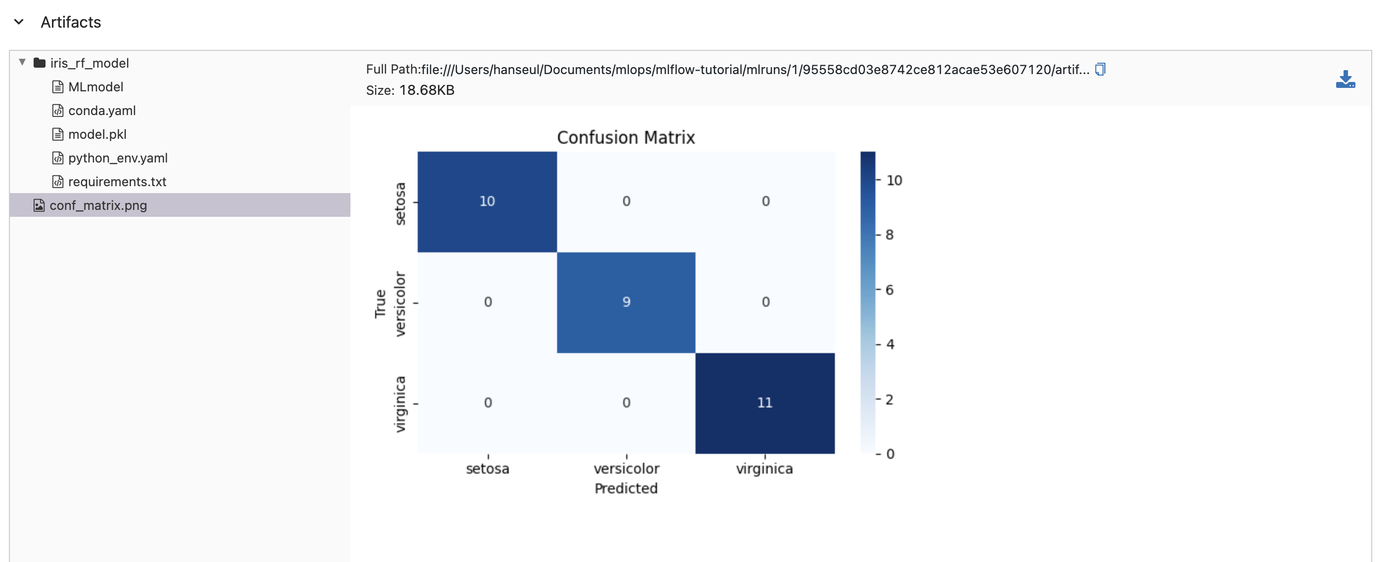
또한, 모델 파일이 정상적으로 저장되어 있는 것도 확인할 수 있습니다.

파일 이름	역할
MLmodel	모델 메타데이터 정의 (저장 형식, 인터페이스, 실행 방법)
conda.yaml	Conda 환경 정의 (Python 버전 및 의존성)
model.pkl	학습된 머신러닝 모델 객체
python_env.yaml	Python 환경 정의
requirements.txt	Pip 의존성 목록 (Python 패키지와 버전 정보)
conf_matrix.png	혼동 행렬 이미지 (모델 성능 평가 결과)

오른쪽에는 mlflow로 저장한 모델을 로드해 사용할 수 있는 예시 코드를 제공합니다.
이 코드를 조금 변형하여 사용해보겠습니다.

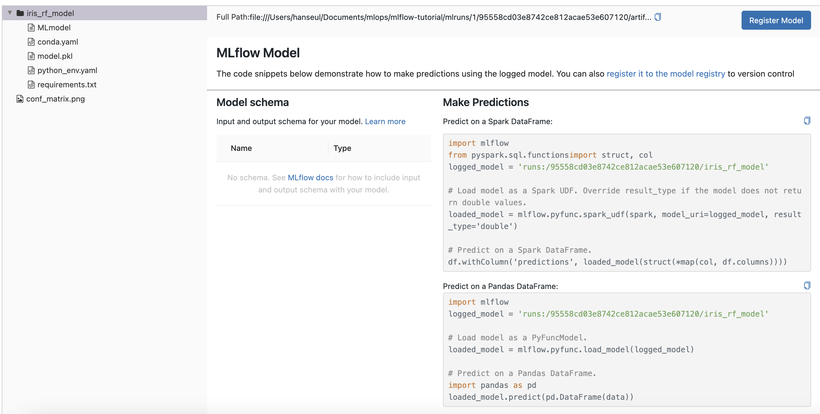
predict.py 파일을 생성해 모델을 로드하고 예측을 수행해봅니다.

# predict.py
import mlflow
import mlflow.pyfunc
import pandas as pd
from sklearn.datasets import load_iris
from sklearn.metrics import accuracy_score, classification_report

iris = load_iris()
data = pd.DataFrame(iris.data, columns=iris.feature_names)
target = iris.target

logged_model = 'runs:/95558cd03e8742ce812acae53e607120/iris_rf_model'

loaded_model = mlflow.pyfunc.load_model(logged_model)

prediction = loaded_model.predict(data)

accuracy = accuracy_score(target, prediction)
report = classification_report(target, prediction)

print(f"Prediction: {prediction}")
print(f"Accuracy: {accuracy:.4f}")
print(report)

결과

Prediction: [0 0 0 0 0 0 0 0 0 0 0 0 0 0 0 0 0 0 0 0 0 0 0 0 0 0 0 0 0 0 0 0 0 0 0 0 0
 0 0 0 0 0 0 0 0 0 0 0 0 0 1 1 1 1 1 1 1 1 1 1 1 1 1 1 1 1 1 1 1 1 2 1 1 1
 1 1 1 2 1 1 1 1 1 2 1 1 1 1 1 1 1 1 1 1 1 1 1 1 1 1 2 2 2 2 2 2 1 2 2 2 2
 2 2 2 2 2 2 2 2 1 2 2 2 2 2 2 2 2 2 2 2 2 2 2 2 2 2 2 2 2 2 2 2 2 2 2 2 2
 2 2]
Accuracy: 0.9667
              precision    recall  f1-score   support

           0       1.00      1.00      1.00        50
           1       0.96      0.94      0.95        50
           2       0.94      0.96      0.95        50

    accuracy                           0.97       150
   macro avg       0.97      0.97      0.97       150
weighted avg       0.97      0.97      0.97       150