[DAY8]_개발일지: Lasso & Tree + forest

1. 학습내용

1. Lasso(최대 반복 횟수 추가)
2. Linear_model(LogisticRegression, 최대 반복횟수 추가)
3. Tree
4. DecisionTreeClassifier
5. DecisionTreeRegressor & LinearRegression
6. RandomForestClassifier
7. GradientBoostingClassifier

2. 주요코드

기본 환경설정

import numpy as np
import pandas as pd
import matplotlib.pyplot as plt

!pip install mglearn

Lasso

from sklearn.linear_model import Lasso

lasso = Lasso().fit(X_train, y_train)

print(lasso.score(X_train, y_train))		#0.29323768991114607
print(lasso.score(X_test, y_test))			#0.20937503255272294

lasso001 = Lasso(alpha=0.01, max_iter=50000).fit(X_train, y_train)

print(lasso001.score(X_train, y_train))		#0.8962226511086497
print(lasso001.score(X_test, y_test))		#0.7656571174549983

# 알파값 기본은 1이며, 1보다 이상일수록 제약이 높아지고 편차는 낮아진다, 훈련정확성은 낮아진다(테스트 정확도는 비교적 높아진다)
# 반대로 1보다 이하일수록, 제약은 낮아지고 편차는 높아진다(데이터가 튄다), 훈련정확성은 높아진다(테스트 정확도는 비교적 낮아진다)

lasso00001 = Lasso(alpha=0.0001, max_iter=50000).fit(X_train, y_train)

print(lasso00001.score(X_train, y_train))		#0.9507158754515467
print(lasso00001.score(X_test, y_test))   		#0.6437467421272709

lasso0 = Lasso(alpha=0, max_iter=50000).fit(X_train, y_train)

  print(lasso0.score(X_train,y_train))			#0.951820862193501
print(lasso0.score(X_test,y_test))				#0.6158830474835724

lasso01 = Lasso(alpha=0.1).fit(X_train, y_train)

print(lasso01.score(X_train, y_train))			#0.7709955157630054
print(lasso01.score(X_test, y_test))			#0.6302009976110041

plt.plot(lasso.coef_, 's', label='Lasso alpha=1', alpha=0.8)
plt.plot(lasso001.coef_, '^', label='Lasso alpha=0.01', alpha=0.5)
plt.plot(lasso00001.coef_, 'v', label='Lasso alpha=0.0001', alpha=0.8)
plt.plot(lasso01.coef_, 'o', label='Lasso alpha=0.1', alpha=0.01)
plt.legend()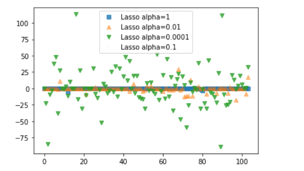

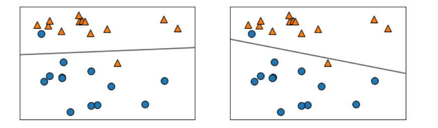
Linear_model(LogisticRegression, 최대 반복횟수 추가)

from sklearn.linear_model import LogisticRegression         #LogisticRegression은 회귀 기법을 이용해서 분류(classification)하는 거
from sklearn.svm import LinearSVC                           #

X, y = mglearn.datasets.make_forge() #샘플데이터 생성

fig, axes = plt.subplots(1, 2, figsize=(10, 3))

for model, ax in zip([LinearSVC(max_iter=5000), LogisticRegression()], axes):
    clf = model.fit(X, y)
    
    mglearn.plots.plot_2d_separator(clf, X, fill=False, eps=0.5, alpha=0.7, ax=ax)
    mglearn.discrete_scatter(X[:,0], X[:,1], y, ax=ax)

mglearn.plots.plot_linear_svc_regularization()           #정규화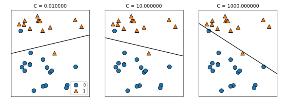

from sklearn.datasets import load_breast_cancer
cancer = load_breast_cancer()

X_train, X_test, y_train, y_test = train_test_split(cancer.data, cancer.target, random_state=42)
logreg = LogisticRegression(max_iter = 5000).fit(X_train, y_train)

print(logreg.score(X_train, y_train))			#0.9624413145539906
print(logreg.score(X_test, y_test))				#0.965034965034965

#L2 제약은 (릿지) 전반적으로 제약을 걸고. 0이 되지 않음                                        #주로 릿지가 정확도가 높아서 자주사용
#L1 제약은 (라쏘) 제약이 쎄면 거의 리니어리그리션에 가까워진다. 0에 가까워질수 있음.

logreg100 = LogisticRegression(max_iter=5000, C=100).fit(X_train, y_train)

print(logreg100.score(X_train, y_train))			#0.9788732394366197	
print(logreg100.score(X_test, y_test))      		#0.965034965034965     

#C 제약은 ALPHA와 반대로 숫자가 클수록 제약이 낮아짐

logreg001 = LogisticRegression(max_iter=5000, C=0.01).fit(X_train, y_train)

print(logreg001.score(X_train, y_train))			#0.9460093896713615
print(logreg001.score(X_test, y_test))     			#0.972027972027972

from sklearn.datasets import make_blobs

X, y = make_blobs(random_state=42)
mglearn.discrete_scatter(X[:,0], X[:,1], y)

plt.xlabel('feature 0')
plt.ylabel('feature 1')
plt.legend(['Class 0','Class 1', 'Class 2'])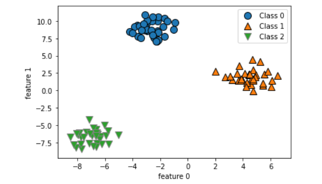

linear_svm = LinearSVC().fit(X, y)

print(linear_svm.coef_)             #기울기
print(linear_svm.coef_.shape)
print(linear_svm.intercept_)        #y절편
print(linear_svm.intercept_.shape)

mglearn.plots.plot_2d_classification(linear_svm, X, fill=True, alpha=0.7) # 색칠범위
mglearn.discrete_scatter(X[:,0], X[:,1], y) #군집범위
line = np.linspace(-15, 15)

for coef, intercept, color in zip(linear_svm.coef_, linear_svm.intercept_, mglearn.cm3.colors):
    plt.plot(line, -(line * coef[0] + intercept) / coef[1], c=color) #그어진 선들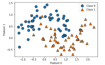

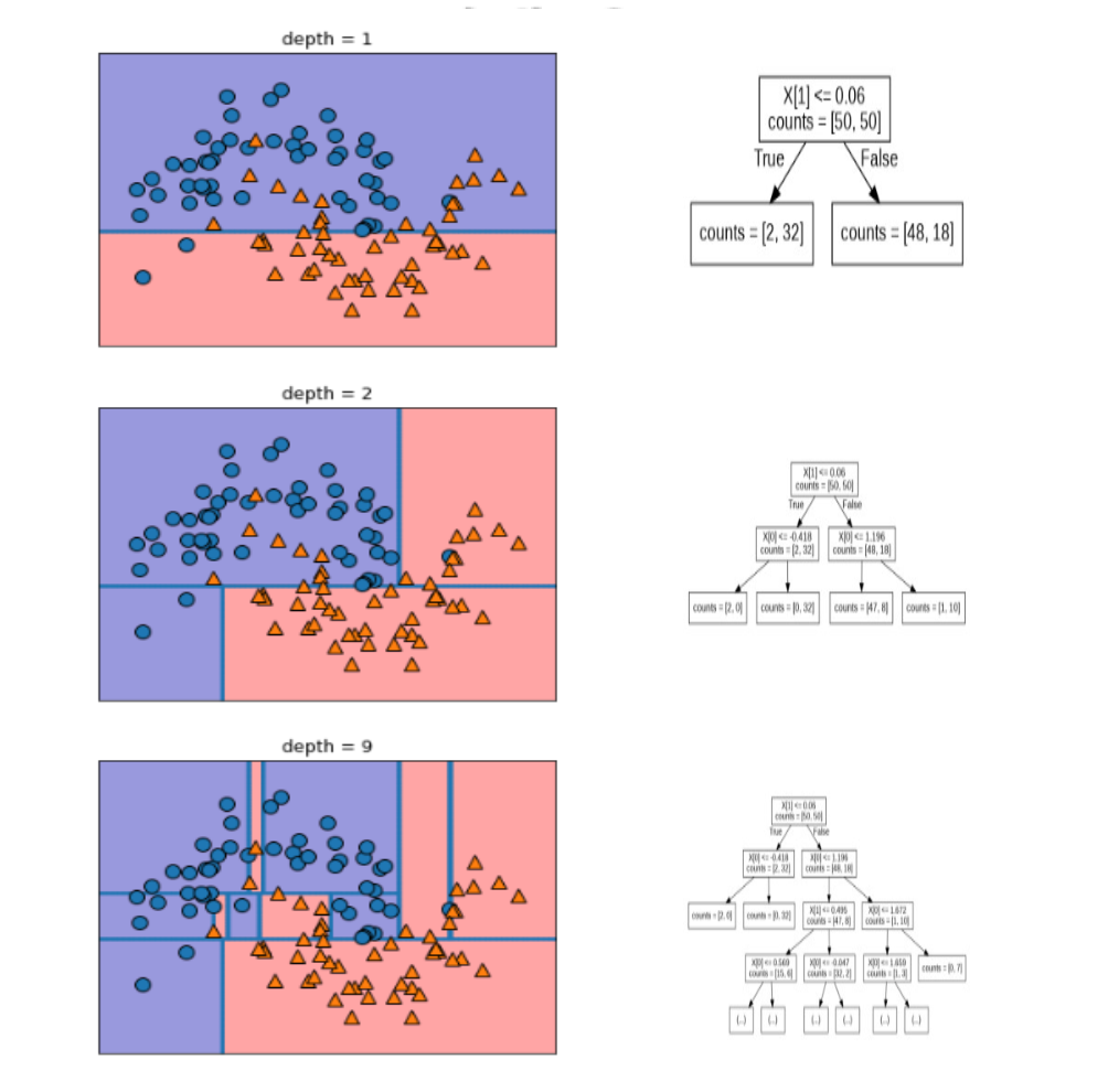
Tree

mglearn.plots.plot_tree_progressive()

DecisionTreeClassifier

from sklearn.tree import DecisionTreeClassifier
from sklearn.datasets import load_breast_cancer

cancer = load_breast_cancer()

X_train, X_test, y_train, y_test = train_test_split(
    cancer.data, cancer.target, random_state=42
)

tree = DecisionTreeClassifier(random_state=0)
tree.fit(X_train, y_train)

print(tree.score(X_train, y_train))			#1.0
print(tree.score(X_test, y_test))			#0.9300699300699301

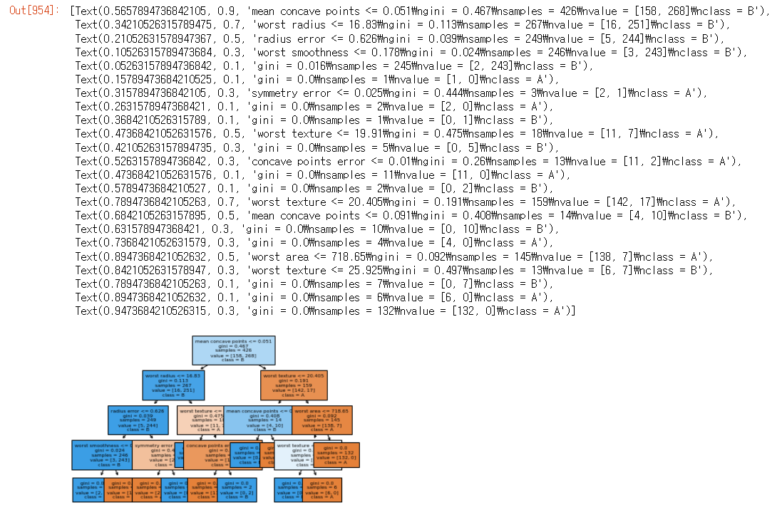
tree = DecisionTreeClassifier(max_depth=4, random_state=0)                 #디폴트보다는 유연하게 트리를 만든다고 볼수있다
tree.fit(X_train, y_train)

print(tree.score(X_train, y_train))			#0.9953051643192489
print(tree.score(X_test, y_test))   		#0.951048951048951

from sklearn.tree import plot_tree            #트리 그리는것

plot_tree(tree, class_names=['A','B'], filled=True, fontsize=6,
         feature_names = cancer.feature_names)

print(tree.feature_importances_)     			           
#뭐가 중요한지 결정이 안나면, 0으로 나타남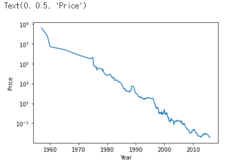

import os
ram_price = pd.read_csv('ram_price.csv')

plt.semilogy(ram_price.date, ram_price.price)
# plt.yticks(fontname = 'Arial')
plt.xlabel('Year')
plt.ylabel('Price')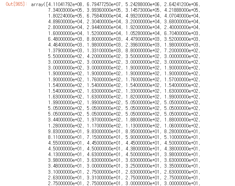

DecisionTreeRegressor & LinearRegression

from sklearn.tree import DecisionTreeClassifier

data_train = ram_price[ram_price.date < 2000]
data_test = ram_price[ram_price.date >= 2000]

X_train = data_train.date.to_numpy()[:,np.newaxis]
y_train = np.log(data_train.price)

from sklearn.tree import DecisionTreeRegressor

tree = DecisionTreeRegressor().fit(X_train, y_train)
linear_reg = LinearRegression().fit(X_train, y_train)

X_all = ram_price.date.to_numpy()[:,np.newaxis]

pred_tree = tree.predict(X_all)
pred_lr = linear_reg.predict(X_all)

price_tree = np.exp(pred_tree)
price_lr = np.exp(pred_lr)

price_tree

(생략)

plt.semilogy(data_train.date, data_train.price, label='Train data')
plt.semilogy(data_test.date, data_test.price, label='Test data')
plt.semilogy(ram_price.date, price_tree, label='Predict tree')
plt.semilogy(ram_price.date, price_lr, label='Predict regression')                  #MAE라고 보면된다

plt.legend()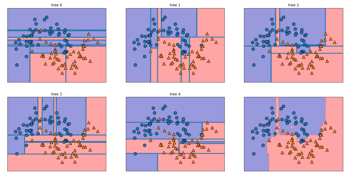

RandomForestClassifier

# RandomForestClassifier

from sklearn.ensemble import RandomForestClassifier
from sklearn.datasets import make_moons

X, y = make_moons(n_samples = 100, noise=0.25, random_state=3)

X_train, X_test, y_train, y_test = train_test_split(X, y, random_state=42)

forest = RandomForestClassifier(n_estimators=5, random_state=2) #100이 default(100개의 나무)
forest.fit(X_train, y_train)

fig, axes = plt.subplots(2,3, figsize=(20, 10))

for i, (ax, tree) in enumerate(zip(axes.ravel(), forest.estimators_)):
    ax.set_title('tree {}'.format(i))
    mglearn.plots.plot_tree_partition(X, y, tree, ax=ax)
    
mglearn.plots.plot_2d_separator(forest, X, fill=True, ax=axes[-1, -1], alpha=0.4)
mglearn.discrete_scatter(X[:,0],X[:,1], y)

X_train, X_test, y_train, y_test = train_test_split(
    cancer.data, cancer.target, random_state=0
)
forest = RandomForestClassifier(n_estimators=100, random_state=0)
forest.fit(X_train, y_train)

print(forest.score(X_train, y_train))			#1.0
print(forest.score(X_test, y_test))				#0.972027972027972

print(forest.feature_importances_)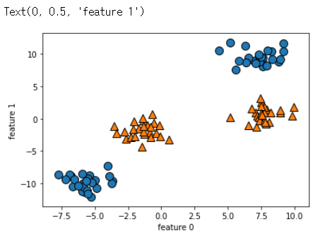

GradientBoostingClassifier

from sklearn.ensemble import GradientBoostingClassifier

X_train, X_test, y_train, y_test = train_test_split(
    cancer.data, cancer.target, random_state=0
)

gbrt = GradientBoostingClassifier(random_state=0)
gbrt.fit(X_train, y_train)

print(gbrt.score(X_train, y_train))				#1.0
print(gbrt.score(X_test, y_test))				#0.965034965034965

gbrt = GradientBoostingClassifier(random_state=0, max_depth=1)     #다음 단계만에 결정함(5까지만해도 충분함), 원하는 결과 빨리, 메모리 적게듬
gbrt.fit(X_train, y_train)

print(gbrt.score(X_train, y_train))				#0.9906103286384976
print(gbrt.score(X_test, y_test))				#0.972027972027972

gbrt = GradientBoostingClassifier(random_state=0, learning_rate = 0.1)
gbrt.fit(X_train, y_train)

print(gbrt.score(X_train, y_train))					#1.0
print(gbrt.score(X_test, y_test))					#0.965034965034965

X, y = make_blobs(centers=4, random_state=8)
y = y % 2

mglearn.discrete_scatter(X[:,0], X[:,1], y)
plt.xlabel('feature 0')
plt.ylabel('feature 1')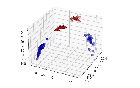

# 두 번째 특성을 제곱하여 추가합니다
X_new = np.hstack([X, X[:, 1:] ** 2])

from mpl_toolkits.mplot3d import Axes3D, axes3d
figure = plt.figure()
# 3차원 그래프
ax = Axes3D(figure, elev=-152, azim=-26)
# y == 0 인 포인트를 먼저 그리고 그 다음 y == 1 인 포인트를 그립니다
mask = y == 0
ax.scatter(X_new[mask, 0], X_new[mask, 1], X_new[mask, 2], c='b',
cmap=mglearn.cm2, s=60, edgecolor='k')
ax.scatter(X_new[~mask, 0], X_new[~mask, 1], X_new[~mask, 2], c='r', marker='^',
cmap=mglearn.cm2, s=60, edgecolor='k')

X_train, X_test, y_train, y_test = train_test_split(
    cancer.data, cancer.target, random_state=0
)

from sklearn.svm import SVC
svc = SVC()
svc.fit(X_train, y_train)

print(svc.score(X_train, y_train))			#0.903755868544601
print(svc.score(X_test, y_test))      		#0.9370629370629371

3. 금일소감

1. 항상 시작할때 'Run All'을 시작할것
2. 코드를 치면서 익숙해지기