[DAY9]_개발일지: Function + 논리게이트

1. 학습내용

1. Jupyter - Function Coding
2. Tensor(텐서)-Vector Coding
3. MNIST 손글씨 이미지 Coding
4. 신경망 논리게이트 Coding - AND
5. 신경망 논리게이트 Coding - OR
6. 신경망 논리게이트 Coding - NAND & XOR

2. 주요코드

기본 환경설정

import math
import numpy as np
import matplotlib.pyplot as plt

plt.style.use('seaborn-whitegrid')

Function(함수) Draw

def linear_function(x):
    a = 0.5
    b = 2
    
    return a * x + b

x = np.arange(-5, 5, 0.1)
y = linear_function(x)

plt.plot(x, y)
plt.xlabel('x')
plt.ylabel('y')
plt.title('Linear Function')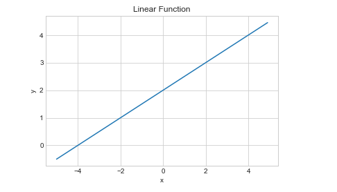

# 2차 함수

def quadratic_function(x):
    a = 1
    b = -2
    c = -2
    
    return a* x**2 + b*x + c

x = np.arange(-5, 5, 0.1)
y = quadratic_function(x)

plt.plot(x, y)
plt.xlabel('x')
plt.ylabel('y')
plt.title('Quadratic Function')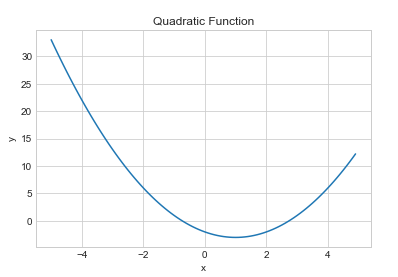

# 3차 함수

def cubic_function(x):
  a = 4
  b = 0
  c = -1
  d = -8

  return a*x**3+b*x**2+c*x+d

x = np.arange(-5, 5, 0.1)
y = cubic_function(x)

plt.plot(x, y)
plt.xlabel('x')
plt.ylabel('y')
plt.title('Cubic Function')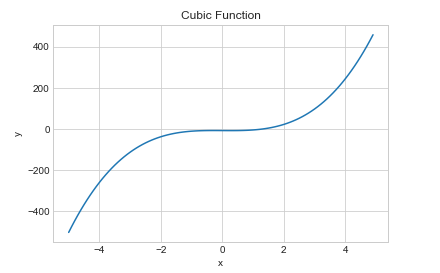

* 교차점 = Check Point

* 텐서는 데이터라고 생각하자!

* 텐서는 5차원 까지! 내용 참고바람

Tensor(텐서)-Vector Coding

#0차원 텐서 스칼라

x = np.array(3)
print(x)					#3
print(x.shape)				#()
print(np.ndim(x))      		#0		 #차원

a = np.array([1,2,3,4])  #어러개의 값이 들어있는 것은 벡터라고 칭함
b = np.array([5,6,7,8])

c = a + b
print(c)					#[ 6  8 10 12]
print(c.shape)				#(4,)
print(np.ndim(c))      		#1	 		#차원

m = np.array(10)        #10이라는 숫자가 하나 들어있는 스칼라 값이라고 칭함
d = a * m
print(d)				[10 20 30 40]

#2차원 텐서의 곲

a = np.array([[1,2,],[3,4]])         #[]를 Parameter로 칭함
b = np.array([[10,10],[10,10]])

print(a)							#[[1 2]
 									 [3 4]]
print(a.shape)						#(2, 2)
print(a.ndim)						#2

print(a * b)						#[[10 20]
 									 [30 40]]

a = np.array([[1,2,3],[4,5,6]])

print(a)						#[[1 2 3]
 								 [4 5 6]]
print(a.shape)					#(2, 3)
print(a.ndim)					#2

# 전치 행렬

a_ = a.T	
print(a_)  							  #[[1 4]
 										[2 5]
 										[3 6]]

X = np.array([[[5,3,2,1],
               [5,5,3,1],
               [6,1,2,3]],
              [[1,1,1,1],
               [3,4,7,5],
               [1,8,3,4]],
              [[10,9,3,9],
               [5,4,3,2],
               [7,6,3,4]]
              ])

print('X\n', X, end='\n\n')
print('X.shape:', X.shape)
print('X.ndim:', X.ndim)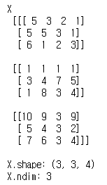

MNIST 손글씨 이미지 분석

#MNIST 손글씨 이미지 분석

!pip install keras
!pip install tensorflow

from keras.datasets import mnist
(X_train, y_train), (X_test, y_test) = mnist.load_data()

print(X_train.shape)				#(60000, 28, 28)
print(X_train.ndim)					#3
print(X_train.dtype)				#uint8

temp_image = X_train[3]

plt.imshow(temp_image, cmap='gray') #컬러값이 들어가면 더 많은 시간이 들어감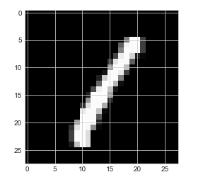

신경망 논리게이트 Coding - AND

import numpy as np
import matplotlib.pyplot as plt
plt.style.use('seaborn-whitegrid')

def AND(x1, x2): 
    input = np.array([x1, x2])             #자극
    weights = np.array([0.4,0.4])          #가중치
    bias = -0.6                            #치우침(편향)
    
    value = np.sum(input * weights) + bias
    
    if value <= 0:
        return 0
    else:
        return 1
    

print(AND(0,0))				#0
print(AND(0,1))				#0
print(AND(1,0))				#0
print(AND(1,1))				#1

x1 = np.arange(-2, 2, 0.01)
x2 = np.arange(-2, 2, 0.01)
bias = -0.6

y = (-0.4 * x1 - bias ) / 0.4

plt.axvline(x=0)          #수직축
plt.axhline(y=0)          #수평축

plt.plot(x1, y, 'r--')
plt.scatter(0,0,color='orange',marker='o',s=150)
plt.scatter(0,1,color='orange',marker='o',s=150)
plt.scatter(1,0,color='orange',marker='o',s=150)
plt.scatter(1,1,color='black',marker='^',s=150)
plt.xlim(-0.5,1.5)
plt.ylim(-0.5,1.5)
plt.grid()

#선을 기준으로 왼쪽은 0, 오른쪽은 1

신경망 논리게이트 Coding - OR

def OR(x1, x2):
  input = np.array([x1, x2])
  weights = np.array([0.4,0.4])
  bias = -0.3

  value = np.sum(input * weights) + bias

  if value <= 0:
    return 0
  else:
    return 1

print(OR(0,0))			#0
print(OR(0,1))			#1
print(OR(1,0))			#1
print(OR(1,1))			#1

x1 = np.arange(-2, 2, 0.01)
x2 = np.arange(-2, 2, 0.01)
bias = -0.3

y = (-0.4 * x1 - bias ) / 0.4               #0.4 는 가중치

plt.axvline(x=0)          #수직축
plt.axhline(y=0)          #수평축

plt.plot(x1, y, 'r--')
plt.scatter(0,0,color='orange',marker='o',s=150)
plt.scatter(0,1,color='orange',marker='^',s=150)
plt.scatter(1,0,color='orange',marker='^',s=150)
plt.scatter(1,1,color='black',marker='^',s=150)
plt.xlim(-0.5,1.5)
plt.ylim(-0.5,1.5)
plt.grid()

#선을 기준으로 왼쪽은 0, 오른쪽은 1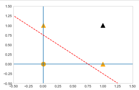

신경망 논리게이트 Coding - NAND & XOR

def NAND(x1, x2):
  input = np.array([x1, x2])
  weights = np.array([-0.6,-0.6])               #가중치와 bias를 수정하면서 논리값을 만든다
  bias = 0.7

  value = np.sum(input * weights) + bias

  if value <= 0:
    return 0
  else:
    return 1

print(NAND(0,0))			#1
print(NAND(0,1))			#1
print(NAND(1,0))			#1
print(NAND(1,1))			#0

def XOR(x1, x2):                      #다층퍼셉트론을 구현하는 수식(인공지능학계의 잃어버린 10년을 깨는 순간)
    s1 = NAND(x1, x2)
    s2 = OR(x1, x2)
    y = AND(s1, s2)
    
    return y

print(XOR(0,0))			#0
print(XOR(0,1))			#1
print(XOR(1,0))			#1
print(XOR(1,1))			#0

keras - 이미지 데이터 쪼개기 후 학습 작업

import keras
keras.__version__

from keras.datasets import mnist
(train_images, train_labels), (test_images, test_labels) = mnist.load_data()         #(xtrain, ytrain) 이라고 생각하면됨

train_images.shape       #(60000, 28, 28)        #총 데이터의 각각의 이미지 자체들
train_labels.shape       #(60000,)       		 #총 데이터의 각각의 이미지 자체들의 숫자들
test_images.shape        #(10000, 28, 28)        #테스트 데이터의 각각의 이미지 자체들
test_labels.shape        #(10000,)       		 #테스트 데이터의 각각의 이미지 자체들의 숫자들

digit = train_images[4]
plt.imshow(digit, cmap='gray')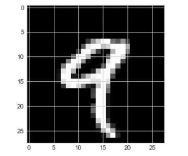

print(train_labels[4])					#9

from keras import models
from keras import layers

network = models.Sequential()
network.add(layers.Dense(512, activation='relu', input_shape = (28 * 28,)))
network.add(layers.Dense(10, activation='softmax'))

3. 금일소감

<ol>
	<li>딥러닝의 시작</li>
	<li>이론은 어렵고 따분했지만, 막상 구현하는 과정에서는 신기하고 재미있었다.</li>
    <li>앞으로가 기대가 된다!</li>
</ol>