개발 환경
- PyCharm을 사용 하였습니다
- Library를 사용 하였습니다(Numpy, matplot, scipy, pandas, cvxpy)
2.1 Library는 PyCharm 내에서 설치할 수 있습니다(File - Settings)
Localization(위치 추정)
예전에는 위치를 알려줄 때 큰 건물이나, 특징적인 것을 기준으로 설명하였다
요즘은 본인이 있는 위치 GPS 값을 보내준다
정의
자동차의 위치를 실시간으로 정확하게 알아내는 기술
자율 주행 자동차에서 가장 핵심적인 Task
정확도를 높이기 위해 다양한 센서 조합과 기법을 사용
필요한 이유
GNSS(GPS 센서를 이용하는 방법)
차량 내비게이션 같은 경우, 길을 알려주는 역할이기 때문에 고정밀할 필요가 없음
but, 자율주행 차량의 경우 현재 위치값을 정확하게 파악하는 것이 중요
차선 폭이 3.2m 정도 되는데 5m의 오차가 있다면 자율주행을 하기 힘듬
차량의 거동 정보만을 사용(Dead reckoning)
Dead reckoning 위치 추종을 하는 경우, 차량 센서에는 오차가 있어 누적 오차가 커짐
보다 정밀한 Localization이 필요함
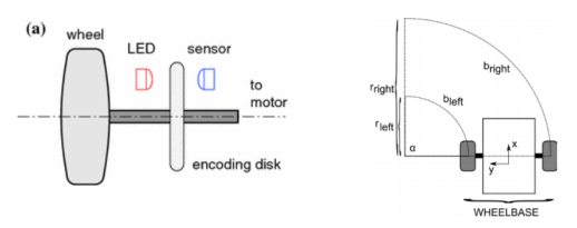
Wheel odometry
정의
바퀴의 회전과 이동 방향을 인코더로 측정하는 방법
오차
시스템 오차
바퀴 지름의 편차, 명목상 수치와 다른 지름을 갖는 바퀴, 명목상 수치와 다른 휠베이스, 정렬되지 않은 바퀴, 인코더 해상도의 한계
비시스템 오차
평평하지 않은 지면에서의 주행, 예상치 못한 장애물을 지나는 주행, 미끄러운 바닥으로 인한 바퀴의 미끄러짐, 급격한 가속이나 회전으로 인한 바퀴의 미끄러짐, 충돌 등으로 인한 외력, 캐스터 휠 등으로 발생하느 내력, 바퀴의 접촉면이 넓은 상황
Dead reckoning(데드 레코닝)
정의
알고 있는 경로를 일정 시간 동안 주행하면서 나온 속도로 간단히 자동차의 현재 위치를 구하는 수학적인 기법
차량에 장착된 주행 기록계와 자기 나침반을 이용
현재는 나침반 대신 각가속도를 측정할 수 있는 압전 센서인 자이로 센서를 이용하여 상대 방향 측정
Wheel encoder
바퀴에 달려 있어 거리나 이동 경로를 측정할 때 사용
종류 : 광학 인코더, 도플러 인코더, 차동 드라이브, 삼륜 드라이브, 애커만 스티어링, 싱크로 드라이브, 전방위 드라이브, 랙 장착 방식...
Ackerman Steering
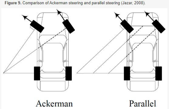
정의
앞 차축 본체를 고정하고 차륜만을 움직여서 변형시키며, 또한 좌우 양륜의 선회 중심이 뒤 차축 중심선 상의 일점에서 만나도록 설계한 것
목적
기하학적 구조로 인하여 타이어의 미끄러짐이 발생하지 않도록 하기 위해 회전축 안쪽 바퀴가 바깥쪽 바퀴보다 더 날카롭게 꺾어지도록 설계
네 바퀴에 동력을 전달하는 자동차에서 주로 사용
Bayes filter
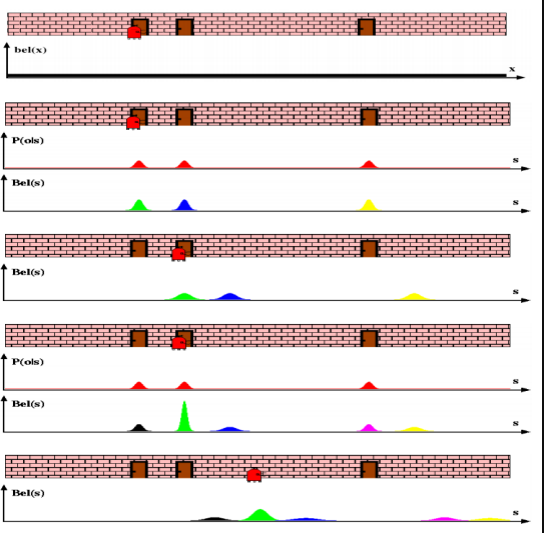
사진 출처 : https://gaussian37.github.io/autodrive-ose-bayes_filter/
Bayes filter를 하기 전에 먼저 베이즈 정리를 보고 가자
Bayes' theorem(베이즈 정리)
정의
이전의 경험과 현재의 증거를 토대로 어떤 사건의 확률을 추론하는 과정
prior과 likelihood를 이용하여 posterior을 구할 수 있음
Bayes filter는 Bayes' theorem을 반복적으로 사용하는 필터로 어떤 사건의 확률을 추론 하는 것을 의미
로봇의 위치에 따라 변화하는 확률을 추론하는 것을 의미
이동 평균 필터
정의
연속된 데이터에서 인접한 n개 데이터의 평균을 구하여 순차적으로 데이터를 필터링
연속된 데이터가 급격하게 변화할 때 이를 완화함
현재의 값에서 미래의 값을 예측할 때 사용함
현재 데이터와 이전의 데이터를 기준으로 구하기 때문에 오차 발생
평균을 구하더라도 오차는 크게 발생함
앞으로의 갈 방향을 예측할 때 사용
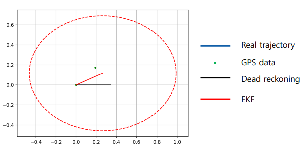
Extended Kalman filter
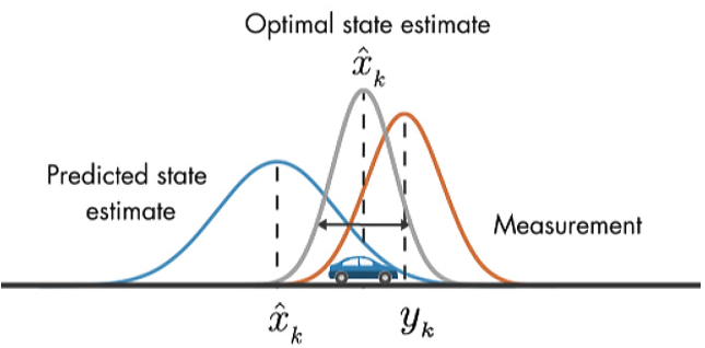
정의
오차를 가지는 관측치로부터 시스템의 상태를 추정하거나 제어하기 위한 알고리즘
시스템이 선형이고 잡음이 정규 분포를 따를 때 사용하기 좋은 필터
일상 생활은 대부분 비선형 -> 칼만 필터 만으로는 한계 존재 -> 확장칼만필터 사용
과정
- 초기값 설정
- 추정 값과 오차 공분산 예측
- 칼만 이득 계산
- 추정값 계산
- 오차 공분산 계산
코드
# main 문에서 실행 해야함
"""

Extended kalman filter (EKF) localization sample

author: Atsushi Sakai (@Atsushi_twi)

"""

import math

import matplotlib.pyplot as plt
import numpy as np

# Covariance for EKF simulation
Q = np.diag([
    0.1,  # variance of location on x-axis
    0.1,  # variance of location on y-axis
    np.deg2rad(1.0),  # variance of yaw angle
    1.0  # variance of velocity
]) ** 2  # predict state covariance
R = np.diag([1.0, 1.0]) ** 2  # Observation x,y position covariance

#  Simulation parameter
INPUT_NOISE = np.diag([1.0, np.deg2rad(30.0)]) ** 2
GPS_NOISE = np.diag([0.5, 0.5]) ** 2

DT = 0.1  # time tick [s]
SIM_TIME = 50.0  # simulation time [s]

show_animation = True


def calc_input():
    v = 1.0  # [m/s]
    yawrate = 0.1  # [rad/s]
    u = np.array([[v], [yawrate]])
    return u

## add def observation
def observation(xTrue, xd, u):
    xTrue = motion_model(xTrue, u)

    # add noise to gps x - y
    z = observation_model(xTrue) + GPS_NOISE @ np.random.randn(2, 1)

    # add noise to input
    ud = u + INPUT_NOISE @ np.random.randn(2, 1)

    xd = motion_model(xd, ud)

    return xTrue, z, xd, ud

## add def motion_model
def motion_model(x, u):
    F = np.array([[1.0, 0, 0, 0],
                  [0, 1.0, 0, 0],
                  [0, 0, 1.0, 0],
                  [0, 0, 0, 0]])

    B = np.array([[DT * math.cos(x[2, 0]), 0],
                  [DT * math.sin(x[2, 0]), 0],
                  [0.0, DT],
                  [1.0, 0.0]])

    x = F @ x + B @ u

    return x

## add def observation_model
def observation_model(x):
    H = np.array([
        [1, 0, 0, 0],
        [0, 1, 0, 0]
    ])

    z = H @ x

    return z

## add def jacob_f
def jacob_f(x, u):
    yaw = x[2, 0]
    v = u[0, 0]
    jF = np.array([
    [1.0, 0.0, -DT * v * math.sin(yaw), DT * math.cos(yaw)],
    [0.0, 1.0, DT * v * math.cos(yaw), DT * math.sin(yaw)],
    [0.0, 0.0, 1.0, 0.0],
    [0.0, 0.0, 0.0, 1.0]])

    return jF

## add def jacob_h
def jacob_h():
    # Jacobian of Observation Model
    jH = np.array([
    [1, 0, 0, 0],
    [0, 1, 0, 0]
    ])

    return jH

## add def ekf_estimation
def ekf_estimation(xEst, PEst, z, u):
    # Predict
    xPred = motion_model(xEst, u)
    jF = jacob_f(xEst, u)
    PPred = jF @ PEst @ jF.T + Q

    # Update
    jH = jacob_h()
    zPred = observation_model(xPred)
    y = z - zPred
    S = jH @ PPred  @ jH.T + R
    K = PPred @ jH.T @ np.linalg.inv(S)
    xEst = xPred + K @ y
    PEst = (np.eye(len(xEst)) - K @ jH) @ PPred
    return xEst, PEst

#add def plot_covariance_ellipse
def plot_covariance_ellipse(xEst, PEst): # pragma : no cover
    Pxy = PEst[0 : 2, 0 : 2]
    eigval, eigvec = np.linalg.eig(Pxy)

    if eigval[0] >= eigval[1]:
        bigind = 0
        smallind = 1
    else:
        bigind = 1
        smallind = 0

    t = np.arange(0, 2 * math.pi + 0.1, 0.1)
    a = math.sqrt(eigval[bigind])
    b = math.sqrt(eigval[smallind])
    x = [a * math.cos(it) for it in t]
    y = [b * math.sin(it) for it in t]
    angle = math.atan2(eigvec[bigind, 1], eigvec[bigind, 0])
    rot = np.array([[math.cos(angle), math.sin(angle)],
                    [-math.sin(angle), math.cos(angle)]])
    fx = rot @ (np.array([x, y]))
    px = np.array(fx[0, :] + xEst[0, 0]).flatten()
    py = np.array(fx[1, :] + xEst[1, 0]).flatten()
    plt.plot(px, py, "--r")

def main():
    print(__file__ + " start!!")

    time = 0.0

    # State Vector [x y yaw v]'
    xEst = np.zeros((4, 1))
    xTrue = np.zeros((4, 1))
    PEst = np.eye(4)

    xDR = np.zeros((4, 1))  # Dead reckoning

    # history
    hxEst = xEst
    hxTrue = xTrue
    hxDR = xTrue
    hz = np.zeros((2, 1))

    while SIM_TIME >= time:
        time += DT
        u = calc_input()

        xTrue, z, xDR, ud = observation(xTrue, xDR, u)

        xEst, PEst = ekf_estimation(xEst, PEst, z, ud)

        # store data history
        hxEst = np.hstack((hxEst, xEst))
        hxDR = np.hstack((hxDR, xDR))
        hxTrue = np.hstack((hxTrue, xTrue))
        hz = np.hstack((hz, z))

        if show_animation:
            plt.cla()
            # for stopping simulation with the esc key.
            plt.gcf().canvas.mpl_connect('key_release_event',
                    lambda event: [exit(0) if event.key == 'escape' else None])
            plt.plot(hz[0, :], hz[1, :], ".g")
            plt.plot(hxTrue[0, :].flatten(),
                     hxTrue[1, :].flatten(), "-b")
            plt.plot(hxDR[0, :].flatten(),
                     hxDR[1, :].flatten(), "-k")
            plt.plot(hxEst[0, :].flatten(),
                     hxEst[1, :].flatten(), "-r")
            plot_covariance_ellipse(xEst, PEst)
            plt.axis("equal")
            plt.grid(True)
            plt.pause(0.001)


if __name__ == '__main__':
    main()
결과
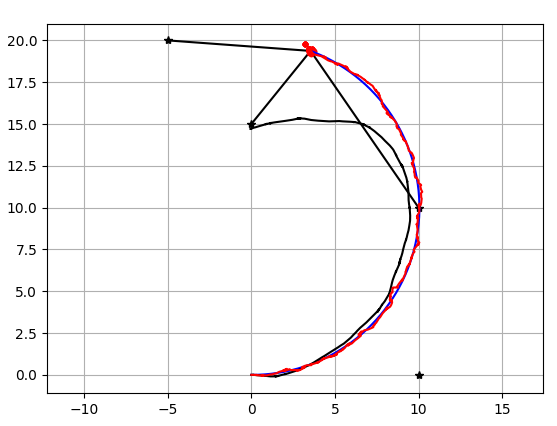
Particle filter localization
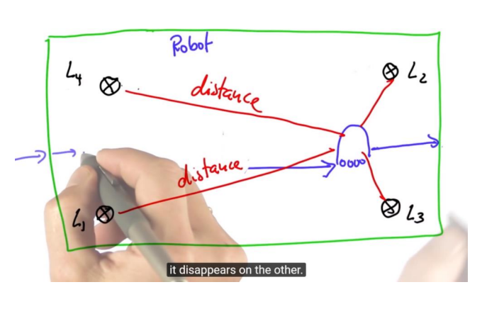
정의
Carlo Localization argorithm이라고도 부름
확률 기반의 위치 추정 기법 중 하나
Histogram, Kalmann Filter와 유사
복잡도를 설정해줄 수 있는 것이 특징
원리
로봇이 이동 명령을 받았을 때, 이동하게 될 위치를 무작위로 생성함 -> 이것을 파티클이라고 부름
현재 환경과 비슷하게 여겨지는 파티클을 생성하는 것을 반복하여 대부분의 파티클이 현재 로봇의 자세와 비슷한 자세의 파티클로 변하게 됨 -> 위치 추정
코드
"""

Particle Filter localization sample

author: Atsushi Sakai (@Atsushi_twi)

"""

import math

import matplotlib.pyplot as plt
import numpy as np
from scipy.spatial.transform import Rotation as Rot

# Estimation parameter of PF
Q = np.diag([0.2]) ** 2  # range error
R = np.diag([2.0, np.deg2rad(40.0)]) ** 2  # input error

#  Simulation parameter
Q_sim = np.diag([0.2]) ** 2
R_sim = np.diag([1.0, np.deg2rad(30.0)]) ** 2

DT = 0.1  # time tick [s]
SIM_TIME = 50.0  # simulation time [s]
MAX_RANGE = 20.0  # maximum observation range

# Particle filter parameter
NP = 100  # Number of Particle
NTh = NP / 2.0  # Number of particle for re-sampling

show_animation = True


def calc_input():
    v = 1.0  # [m/s]
    yaw_rate = 0.1  # [rad/s]
    u = np.array([[v, yaw_rate]]).T
    return u


def observation(x_true, xd, u, rf_id):
    x_true = motion_model(x_true, u)

    # add noise to gps x-y
    z = np.zeros((0, 3))

    for i in range(len(rf_id[:, 0])):

        dx = x_true[0, 0] - rf_id[i, 0]
        dy = x_true[1, 0] - rf_id[i, 1]
        d = math.hypot(dx, dy)
        if d <= MAX_RANGE:
            dn = d + np.random.randn() * Q_sim[0, 0] ** 0.5  # add noise
            zi = np.array([[dn, rf_id[i, 0], rf_id[i, 1]]])
            z = np.vstack((z, zi))

    # add noise to input
    ud1 = u[0, 0] + np.random.randn() * R_sim[0, 0] ** 0.5
    ud2 = u[1, 0] + np.random.randn() * R_sim[1, 1] ** 0.5
    ud = np.array([[ud1, ud2]]).T

    xd = motion_model(xd, ud)

    return x_true, z, xd, ud

## add def motion_model
def motion_model(x, u):
    F = np.array([[1.0, 0, 0, 0],
                  [0, 1.0, 0, 0],
                  [0, 0, 1.0, 0],
                  [0, 0, 0, 0]])
    B = np.array([[DT * math.cos(x[2, 0]), 0],
                  [DT * math.sin(x[2, 0]), 0],
                  [0.0, DT],
                  [1.0, 0.0]])

    x = F.dot(x) + B.dot(u)

    return x

## add def gauss_likelihood
def gauss_likelihood(x, sigma):
    p = 1.0 / math.sqrt(2.0 * math.pi * sigma ** 2) * \
        math.exp(-x ** 2 / (2 * sigma ** 2))
    return p

## add def calc_covariance
def calc_covariance(x_est, px, pw):
    """
    calculate covariance matrix
    see ipynb doc
    """
    cov = np.zeros((3, 3))
    n_particle = px.shape[1]
    for i in range(n_particle):
        dx = (px[:, i:i + 1] - x_est)[0:3]
        cov += pw[0, i] * dx @ dx.T
    cov *= 1.0 / (1.0 - pw @ pw.T)

    return cov


#### add def pf_localization
def pf_localization(px, pw, z, u):
    """
    Localization with Particle filter
    """

    for ip in range(NP):
        x = np.array([px[:, ip]]).T
        w = pw[0, ip]

        # Predict with random input sampling
        ud1 = u[0, 0] + np.random.randn() * R[0, 0] ** 0.5
        ud2 = u[1, 0] + np.random.randn() * R[1, 1] ** 0.5
        ud = np.array([[ud1, ud2]]).T
        x = motion_model(x, ud)

        # Calc Importance Weight
        for i in range(len(z[:, 0])):
            dx = x[0, 0] - z[i, 1]
            dy = x[1, 0] - z[i, 2]
            pre_z = math.hypot(dx, dy)
            dz = pre_z - z[i, 0]
            w = w * gauss_likelihood(dz, math.sqrt(Q[0, 0]))

        px[:, ip] = x[:, 0]
        pw[0, ip] = w

    pw = pw / pw.sum() # normalize
    x_est = px.dot(pw.T)
    p_est = calc_covariance(x_est, px, pw)
    N_eff = 1.0 / (pw.dot(pw.T))[0, 0] # Effective particle number

    if N_eff < NTh:
        px, pw = re_sampling(px, pw)

    return x_est, p_est, px, pw


### add def re_sampling
def re_sampling(px, pw):
    """
    low variance re-sampling
    """
    w_cum = np.cumsum(pw)
    base = np.arange(0.0, 1.0, 1 / NP)
    re_sample_id = base + np.random.uniform(0, 1 / NP)
    indexes = []
    ind = 0
    for ip in range(NP):
        while re_sample_id[ip] > w_cum[ind]:
            ind += 1
        indexes.append(ind)

    px = px[:, indexes]
    pw = np.zeros((1, NP)) + 1.0 / NP # init weight

    return px, pw


def plot_covariance_ellipse(x_est, p_est):  # pragma: no cover
    p_xy = p_est[0:2, 0:2]
    eig_val, eig_vec = np.linalg.eig(p_xy)

    if eig_val[0] >= eig_val[1]:
        big_ind = 0
        small_ind = 1
    else:
        big_ind = 1
        small_ind = 0

    t = np.arange(0, 2 * math.pi + 0.1, 0.1)

    # eig_val[big_ind] or eiq_val[small_ind] were occasionally negative
    # numbers extremely close to 0 (~10^-20), catch these cases and set the
    # respective variable to 0
    try:
        a = math.sqrt(eig_val[big_ind])
    except ValueError:
        a = 0

    try:
        b = math.sqrt(eig_val[small_ind])
    except ValueError:
        b = 0

    x = [a * math.cos(it) for it in t]
    y = [b * math.sin(it) for it in t]
    angle = math.atan2(eig_vec[big_ind, 1], eig_vec[big_ind, 0])
    rot = Rot.from_euler('z', angle).as_matrix()[0:2, 0:2]
    fx = rot.dot(np.array([[x, y]]))
    px = np.array(fx[0, :] + x_est[0, 0]).flatten()
    py = np.array(fx[1, :] + x_est[1, 0]).flatten()
    plt.plot(px, py, "--r")


def main():
    print(__file__ + " start!!")

    time = 0.0

    # RF_ID positions [x, y]
    rf_id = np.array([[10.0, 0.0],
                      [10.0, 10.0],
                      [0.0, 15.0],
                      [-5.0, 20.0]])

    # State Vector [x y yaw v]'
    x_est = np.zeros((4, 1))
    x_true = np.zeros((4, 1))

    px = np.zeros((4, NP))  # Particle store
    pw = np.zeros((1, NP)) + 1.0 / NP  # Particle weight
    x_dr = np.zeros((4, 1))  # Dead reckoning

    # history
    h_x_est = x_est
    h_x_true = x_true
    h_x_dr = x_true

    while SIM_TIME >= time:
        time += DT
        u = calc_input()

        x_true, z, x_dr, ud = observation(x_true, x_dr, u, rf_id)

        x_est, PEst, px, pw = pf_localization(px, pw, z, ud)

        # store data history
        h_x_est = np.hstack((h_x_est, x_est))
        h_x_dr = np.hstack((h_x_dr, x_dr))
        h_x_true = np.hstack((h_x_true, x_true))

        if show_animation:
            plt.cla()
            # for stopping simulation with the esc key.
            plt.gcf().canvas.mpl_connect(
                'key_release_event',
                lambda event: [exit(0) if event.key == 'escape' else None])

            for i in range(len(z[:, 0])):
                plt.plot([x_true[0, 0], z[i, 1]], [x_true[1, 0], z[i, 2]], "-k")
            plt.plot(rf_id[:, 0], rf_id[:, 1], "*k")
            plt.plot(px[0, :], px[1, :], ".r")
            plt.plot(np.array(h_x_true[0, :]).flatten(),
                     np.array(h_x_true[1, :]).flatten(), "-b")
            plt.plot(np.array(h_x_dr[0, :]).flatten(),
                     np.array(h_x_dr[1, :]).flatten(), "-k")
            plt.plot(np.array(h_x_est[0, :]).flatten(),
                     np.array(h_x_est[1, :]).flatten(), "-r")
            plot_covariance_ellipse(x_est, PEst)
            plt.axis("equal")
            plt.grid(True)
            plt.pause(0.001)


if __name__ == '__main__':
    main()
결과
알고리즘 종류
- Dijkstra algorithm
- A* algorithm
- Optimal Trajectory in a Frenet Frame
Dijkstra algorithm
정의
그래프 이론에서 대표적으로 손꼽히는 최단 경로 알고리즘
1959년에 에츠허르 데이크스트라가 제안함
가중치 그래프(Weighted graph)에서 최단 경로 계산
원리
사진 출처 : https://www.codingame.com/learn/pathfinding
- 차로 지점에 대한 연결 그래프 구성 -> 가까운 지점 출발, 목적지 노드 설정
- 출발 차로 지점 설정 -> 방문하지 않은 지점 미방문의 집합에 포함 -> 차로 지점과 그 차로 지점 이전에 나온 선행 차로 지점의 최단 거리로 맵 작성
- 현재 차로 지점에 인접한 미방문 차로 지점에 대해 잠재 거리를 계산 -> 거리의 크기를 비교하여 유지 또는 대체 -> 맵 갱신
- 위의 3번째 단계를 인접 미방문 차로로 대해 반복, 모든 인접 지점에 작업이 끝나면 현재 노드를 방문 노드로 표시한 뒤 미방문 집합에서 제거
- 목적 차로 지점이 미방문 지점에서 제거되거나, 무한대의 잠재 거리를 가지고 있으면 끝남
코드
"""
Grid based Dijkstra planning
author: Atsushi Sakai(@Atsushi_twi)
"""
import matplotlib.pyplot as plt
import math
show_animation = True
class Dijkstra:
def __init__(self, ox, oy, resolution, robot_radius):
"""
Initialize map for a star planning
ox: x position list of Obstacles [m]
oy: y position list of Obstacles [m]
resolution: grid resolution [m]
rr: robot radius[m]
"""
self.min_x = None
self.min_y = None
self.max_x = None
self.max_y = None
self.x_width = None
self.y_width = None
self.obstacle_map = None
self.resolution = resolution
self.robot_radius = robot_radius
self.calc_obstacle_map(ox, oy)
self.motion = self.get_motion_model()
class Node:
def __init__(self, x, y, cost, parent_index):
self.x = x # index of grid
self.y = y # index of grid
self.cost = cost
self.parent_index = parent_index # index of previous Node
def __str__(self):
return str(self.x) + "," + str(self.y) + "," + str(
self.cost) + "," + str(self.parent_index)
## add def planning
def planning(self, sx, sy, gx, gy):
start_node = self.Node(self.calc_xy_index(sx, self.min_x),
self.calc_xy_index(sy, self.min_y), 0.0, -1)
goal_node = self.Node(self.calc_xy_index(gx, self.min_x),
self.calc_xy_index(gy, self.min_y), 0.0, -1)
open_set, closed_set = dict(), dict()
open_set[self.calc_index(start_node)] = start_node
while 1:
c_id = min(open_set, key=lambda o: open_set[o].cost)
current = open_set[c_id]
# show graph
if show_animation: # pragma: no cover
plt.plot(self.calc_position(current.x, self.min_x),
self.calc_position(current.y, self.min_y), "xc")
# for stopping simulation with the esc key.
plt.gcf().canvas.mpl_connect(
'key_release_event',
lambda event: [exit(0) if event.key == 'escape' else None])
if len(closed_set.keys()) % 10 == 0:
plt.pause(0.001)
if current.x == goal_node.x and current.y == goal_node.y:
print("Find goal")
goal_node.parent_index = current.parent_index
goal_node.cost = current.cost
break
# Remove the item from the open set
del open_set[c_id]
# Add it to the closed set
closed_set[c_id] = current
# expand search grid based on motion model
for move_x, move_y, move_cost in self.motion:
node = self.Node(current.x + move_x,
current.y + move_y,
current.cost + move_cost, c_id)
n_id = self.calc_index(node)
if n_id in closed_set:
continue
if not self.verify_node(node):
continue
if n_id not in open_set:
open_set[n_id] = node # Discover a new node
else:
if open_set[n_id].cost >= node.cost:
# This path is the best until now. record it!
open_set[n_id] = node
rx, ry = self.calc_final_path(goal_node, closed_set)
return rx, ry
## add def calc_final_path
def calc_final_path(self, goal_node, closed_set):
# generate final course
rx, ry = [self.calc_position(goal_node.x, self.min_x)], [self.calc_position(goal_node.y, self.min_y)]
parent_index = goal_node.parent_index
while parent_index != -1:
n = closed_set[parent_index]
rx.append(self.calc_position(n.x, self.min_x))
ry.append(self.calc_position(n.y, self.min_y))
parent_index = n.parent_index
return rx, ry
def calc_position(self, index, minp):
pos = index * self.resolution + minp
return pos
def calc_xy_index(self, position, minp):
return round((position - minp) / self.resolution)
def calc_index(self, node):
return (node.y - self.min_y) * self.x_width + (node.x - self.min_x)
def verify_node(self, node):
px = self.calc_position(node.x, self.min_x)
py = self.calc_position(node.y, self.min_y)
if px < self.min_x:
return False
if py < self.min_y:
return False
if px >= self.max_x:
return False
if py >= self.max_y:
return False
if self.obstacle_map[node.x][node.y]:
return False
return True
def calc_obstacle_map(self, ox, oy):
self.min_x = round(min(ox))
self.min_y = round(min(oy))
self.max_x = round(max(ox))
self.max_y = round(max(oy))
print("min_x:", self.min_x)
print("min_y:", self.min_y)
print("max_x:", self.max_x)
print("max_y:", self.max_y)
self.x_width = round((self.max_x - self.min_x) / self.resolution)
self.y_width = round((self.max_y - self.min_y) / self.resolution)
print("x_width:", self.x_width)
print("y_width:", self.y_width)
# obstacle map generation
self.obstacle_map = [[False for _ in range(self.y_width)]
for _ in range(self.x_width)]
for ix in range(self.x_width):
x = self.calc_position(ix, self.min_x)
for iy in range(self.y_width):
y = self.calc_position(iy, self.min_y)
for iox, ioy in zip(ox, oy):
d = math.hypot(iox - x, ioy - y)
if d <= self.robot_radius:
self.obstacle_map[ix][iy] = True
break
@staticmethod
def get_motion_model():
# dx, dy, cost
motion = [[1, 0, 1],
[0, 1, 1],
[-1, 0, 1],
[0, -1, 1],
[-1, -1, math.sqrt(2)],
[-1, 1, math.sqrt(2)],
[1, -1, math.sqrt(2)],
[1, 1, math.sqrt(2)]]
return motion
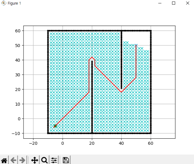
def main():
print(__file__ + " start!!")
# start and goal position
sx = -5.0 # [m]
sy = -5.0 # [m]
gx = 50.0 # [m]
gy = 50.0 # [m]
grid_size = 2.0 # [m]
robot_radius = 1.0 # [m]
# set obstacle positions
ox, oy = [], []
for i in range(-10, 60):
ox.append(i)
oy.append(-10.0)
for i in range(-10, 60):
ox.append(60.0)
oy.append(i)
for i in range(-10, 61):
ox.append(i)
oy.append(60.0)
for i in range(-10, 61):
ox.append(-10.0)
oy.append(i)
for i in range(-10, 40):
ox.append(20.0)
oy.append(i)
for i in range(0, 40):
ox.append(40.0)
oy.append(60.0 - i)
if show_animation: # pragma: no cover
plt.plot(ox, oy, ".k")
plt.plot(sx, sy, "og")
plt.plot(gx, gy, "xb")
plt.grid(True)
plt.axis("equal")
dijkstra = Dijkstra(ox, oy, grid_size, robot_radius)
rx, ry = dijkstra.planning(sx, sy, gx, gy)
if show_animation: # pragma: no cover
plt.plot(rx, ry, "-r")
plt.pause(0.01)
plt.show()
if __name__ == '__main__':
main()결과
A* algorithm(A star algorithm)
정의
데이크스트라 알고리즘을 확장한 휴리스틱(Huristic)기반 최적 우선 탐색 알고리즘
Dijkstra algorithm과 마찬가지로 흔히 사용됨
데이크스트라 알고리즘도 인 A* 알고리즘이라 할 수 있음
원리
- 가치 기반(merit - based)또는 최적 우선(best-first)탐색 알고리즘
- Openset 노드 집합을 이용하여 잠재 노드를 담음
- 노드의 비용
- = 출발 노드에서의 비용 = 현재 노드에서 목적에 이르는 최소 비용 추정치
- A* 탐색 과정에서 루프를 돌 때마다 목적 노드가 확장될 때 까지 최소 비용이 인 노드가 확장
코드
"""
A* grid planning
author: Atsushi Sakai(@Atsushi_twi)
Nikos Kanargias (nkana@tee.gr)
See Wikipedia article (https://en.wikipedia.org/wiki/A*_search_algorithm)
"""
import math
import matplotlib.pyplot as plt
show_animation = True
class AStarPlanner:
def __init__(self, ox, oy, resolution, rr):
"""
Initialize grid map for a star planning
ox: x position list of Obstacles [m]
oy: y position list of Obstacles [m]
resolution: grid resolution [m]
rr: robot radius[m]
"""
self.resolution = resolution
self.rr = rr
self.min_x, self.min_y = 0, 0
self.max_x, self.max_y = 0, 0
self.obstacle_map = None
self.x_width, self.y_width = 0, 0
self.motion = self.get_motion_model()
self.calc_obstacle_map(ox, oy)
class Node:
def __init__(self, x, y, cost, parent_index):
self.x = x # index of grid
self.y = y # index of grid
self.cost = cost
self.parent_index = parent_index
def __str__(self):
return str(self.x) + "," + str(self.y) + "," + str(
self.cost) + "," + str(self.parent_index)
##add def planning
def planning(self, sx, sy, gx, gy):
"""
A star path search
input:
s_x: start x position [m]
s_y: start y position [m]
gx: goal x position [m]
gy: goal y position [m]
output:
rx: x position list of the final path
ry: y position list of the final path
"""
start_node = self.Node(self.calc_xy_index(sx, self.min_x),
self.calc_xy_index(sy, self.min_y), 0.0, -1)
goal_node = self.Node(self.calc_xy_index(gx, self.min_x),
self.calc_xy_index(gy, self.min_y), 0.0, -1)
open_set, closed_set = dict(), dict()
open_set[self.calc_grid_index(start_node)] = start_node
while 1:
if len(open_set) == 0:
print("Open set is empty..")
break
c_id = min(
open_set,
key=lambda o: open_set[o].cost + self.calc_heuristic(goal_node,
open_set[
o]))
current = open_set[c_id]
# show graph
if show_animation: # pragma: no cover
plt.plot(self.calc_grid_position(current.x, self.min_x),
self.calc_grid_position(current.y, self.min_y), "xc")
# for stopping simulation with the esc key.
plt.gcf().canvas.mpl_connect('key_release_event',
lambda event: [exit(
0) if event.key == 'escape' else None])
if len(closed_set.keys()) % 10 == 0:
plt.pause(0.001)
if current.x == goal_node.x and current.y == goal_node.y:
print("Find goal")
goal_node.parent_index = current.parent_index
goal_node.cost = current.cost
break
# Remove the item from the open set
del open_set[c_id]
# Add it to the closed set
closed_set[c_id] = current
# expand_grid search grid based on motion model
for i, _ in enumerate(self.motion):
node = self.Node(current.x + self.motion[i][0],
current.y + self.motion[i][1],
current.cost + self.motion[i][2], c_id)
n_id = self.calc_grid_index(node)
# If the node is not safe, do nothing
if not self.verify_node(node):
continue
if n_id in closed_set:
continue
if n_id not in open_set:
open_set[n_id] = node # discovered a new node
else:
if open_set[n_id].cost > node.cost:
# This path is the best until now. record it
open_set[n_id] = node
rx, ry = self.calc_final_path(goal_node, closed_set)
return rx, ry
def calc_final_path(self, goal_node, closed_set):
# generate final course
rx, ry = [self.calc_grid_position(goal_node.x, self.min_x)], [
self.calc_grid_position(goal_node.y, self.min_y)]
parent_index = goal_node.parent_index
while parent_index != -1:
n = closed_set[parent_index]
rx.append(self.calc_grid_position(n.x, self.min_x))
ry.append(self.calc_grid_position(n.y, self.min_y))
parent_index = n.parent_index
return rx, ry
@staticmethod
def calc_heuristic(n1, n2):
w = 1.0 # weight of heuristic
d = w * math.hypot(n1.x - n2.x, n1.y - n2.y)
return d
def calc_grid_position(self, index, min_position):
"""
calc grid position
:param index:
:param min_position:
:return:
"""
pos = index * self.resolution + min_position
return pos
def calc_xy_index(self, position, min_pos):
return round((position - min_pos) / self.resolution)
def calc_grid_index(self, node):
return (node.y - self.min_y) * self.x_width + (node.x - self.min_x)
def verify_node(self, node):
px = self.calc_grid_position(node.x, self.min_x)
py = self.calc_grid_position(node.y, self.min_y)
if px < self.min_x:
return False
elif py < self.min_y:
return False
elif px >= self.max_x:
return False
elif py >= self.max_y:
return False
# collision check
if self.obstacle_map[node.x][node.y]:
return False
return True
def calc_obstacle_map(self, ox, oy):
self.min_x = round(min(ox))
self.min_y = round(min(oy))
self.max_x = round(max(ox))
self.max_y = round(max(oy))
print("min_x:", self.min_x)
print("min_y:", self.min_y)
print("max_x:", self.max_x)
print("max_y:", self.max_y)
self.x_width = round((self.max_x - self.min_x) / self.resolution)
self.y_width = round((self.max_y - self.min_y) / self.resolution)
print("x_width:", self.x_width)
print("y_width:", self.y_width)
# obstacle map generation
self.obstacle_map = [[False for _ in range(self.y_width)]
for _ in range(self.x_width)]
for ix in range(self.x_width):
x = self.calc_grid_position(ix, self.min_x)
for iy in range(self.y_width):
y = self.calc_grid_position(iy, self.min_y)
for iox, ioy in zip(ox, oy):
d = math.hypot(iox - x, ioy - y)
if d <= self.rr:
self.obstacle_map[ix][iy] = True
break
@staticmethod
def get_motion_model():
# dx, dy, cost
motion = [[1, 0, 1],
[0, 1, 1],
[-1, 0, 1],
[0, -1, 1],
[-1, -1, math.sqrt(2)],
[-1, 1, math.sqrt(2)],
[1, -1, math.sqrt(2)],
[1, 1, math.sqrt(2)]]
return motion
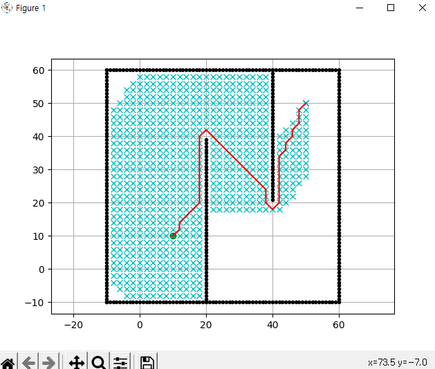
def main():
print(__file__ + " start!!")
# start and goal position
sx = 10.0 # [m]
sy = 10.0 # [m]
gx = 50.0 # [m]
gy = 50.0 # [m]
grid_size = 2.0 # [m]
robot_radius = 1.0 # [m]
# set obstacle positions
ox, oy = [], []
for i in range(-10, 60):
ox.append(i)
oy.append(-10.0)
for i in range(-10, 60):
ox.append(60.0)
oy.append(i)
for i in range(-10, 61):
ox.append(i)
oy.append(60.0)
for i in range(-10, 61):
ox.append(-10.0)
oy.append(i)
for i in range(-10, 40):
ox.append(20.0)
oy.append(i)
for i in range(0, 40):
ox.append(40.0)
oy.append(60.0 - i)
if show_animation: # pragma: no cover
plt.plot(ox, oy, ".k")
plt.plot(sx, sy, "og")
plt.plot(gx, gy, "xb")
plt.grid(True)
plt.axis("equal")
a_star = AStarPlanner(ox, oy, grid_size, robot_radius)
rx, ry = a_star.planning(sx, sy, gx, gy)
if show_animation: # pragma: no cover
plt.plot(rx, ry, "-r")
plt.pause(0.001)
plt.show()
if __name__ == '__main__':
main()결과

너무멋져요