1. Control system engineering(Introduction)

이준혁·2026년 2월 9일

control system

해당 글은 개인적으로 공부하기 위한 글로 알아주시면 감사하겠습니다.

1.시스템 구조

개루프 시스템

개루프 시스템은 입력 명령을 제어하기에 적합한 형태로 변환하는 입력변환기(input transducer)라는 보조 시스템으로 시작함
입력은 기준입력(reference)로 칭하며 출력은 피제어 변수(controlled variable)라고 칭함
외란과 같은 신호는 입력되는 신호들을 대수적으로 합하는 접합점(summing junction)에서 제어기나 공정의 출력과 합해짐
질량이 움직일때 일정한 힘을 소모하는 제동기(damper)와 질량 및 스프링으로 구성되는 기계 시스템은 또 다른 개루프 시스템의 한 예임
개루프는 외란에 민감하여 외란을 제거하지 못하는 것이 단점

폐루프 시스템(feedback system)

입력 변환기는 입력 명령을 제어기에 적합한 형태로 변환시키며 출력변환기(output transducer) 또는 센서(sensor)로 출력을 측정하여 제어기에 적합한 형태로 변환
접합점으로 피드백 경로(feedback path)을 통하여 도달하는 출력 신호와 입력 신호를 대수적으로 합함
출력 신호의 부호가 반전되어 신호가 합해지는데 이를 구동신호(actuating signal)이라고 함
실제 입력과 출력의 차가 구동 신호가 되는데이를 오차(error) 라고 함
간단한 이득 조정을 하거나 제어기를 재설계함으로 써 과도 응답과 정상 상태 오차를 개선시키는것을 보상(compensating)이라고 함 재설계된 하드웨어를 보상기(compensator)라고 함

2. 해석과 설계 목적

과도 응답

과도 응답이 너무 빠르면 복구하지 못할 물리적 손상을 시스템에 입힐수 있음

정상상태 응답

안정도

과도 응답과 정상 상태 오차에 대한 해석과 설계는 시스템이 안정하지 않는 경우에는 의미가 없음
고유응답(natural response)과 강제응답(foreced responser)의 합으로 표시됨
이런 응답을 각각 동차해(homogeneous solution), 특이해(particular solution)이라함
선형시스템은 전체 응답의 다음과 같이 표현됨 $전체 응답 = 고유 응답 + 강제응답$

사례연구

이런 진동하거나 정상 상태에서는 고유응답이 0으로 되어 강제응답만 남는 경우 불안정(instability)라고 함
감쇠진동(daped oscillation) : 시간에 따라 크기가 줄어드는 정현파 응답하는 과도 상태를 갖게 되는것

3. 설계 절차

1단계 : 요구조건에 맞는 실제 시스템 선정

요구 조건에 맞는 실제 시스템(physical system)을 선정함

2단계 : 기능별 블럭선도 작성

정상적으로 표현된 시스템의 각 부분을 기능별 블록선도로 나타내고 이를 블록들을 상호 연결하여 전체 블록선도를 완성함

3단계 : 구조 개요도 도안

예로 직류전동기(dc motor) 구동 시키기 위해 차동 증폭기(differential amplifier)와 전력 증폭기는 각각 이득이나 전력 증폭을 하는 제어기로 사용됨
부하(load)의 경우 회전하는 질량과 베어링 마찰을 가지므로 부하 모델은 자동차의 충격 흡수 장치나 스크린 문 제동기(screen door damper)와 같이 속도와 증가함에 따라 역회전 토크(torque)가 증가되는 관성(inertia)와 점성마찰(viscous damping)으로 표현됨

4단계 : 수학적 모델의 개발

시스템 구조에 대한 개요도가 완성되면 전기 회로에 kirchhoff의 법칙과 실제 시스템에 대해 적용되는 Newton의 법칙과 같은 물리적 법칙과 가정을 이용하여 시스템을 모델링함
kirchhoff의 전압 / 전류 법칙, newton의 법칙을 이용하면서 동적 시스템의 입력과 출력 사이의 관계를 나타내는 수학적 모델링을 얻을수 있음
선형 시불변 미분방정식(linear time-invariant differential equation)으로 표시됨
시스템 모델은 차수가 높아지거나 비선형 시변(nonlinear time varying) 또는 편미분 방정식(partial differential equation)으로 표현됨
전달함수(transfer function)은 시스템을 수학적으로 모델링하는 방법으로 전달함수를 laplace변환을 이용하여 선형 시불변 미분방정식으로 유도됨
상태공간(state space)에서도 시스템 모델이 표현될수 있음 이는 모델을 상태 공간에서 표현하려는 이유는 선형 미분 방정식으로 나타낼수 없는 시스템에서도 적용할수 있을 뿐만 아니라 시뮬레이션하기 편한 형태로 나타낼수 있기 때문

5단계 : 블럭선도 단순화

6단계 : 해석과 설계

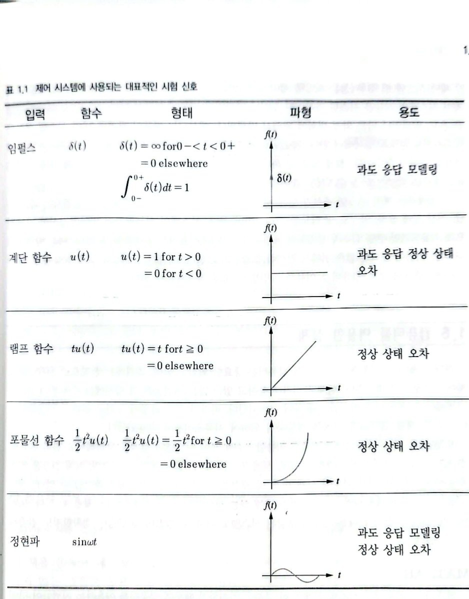
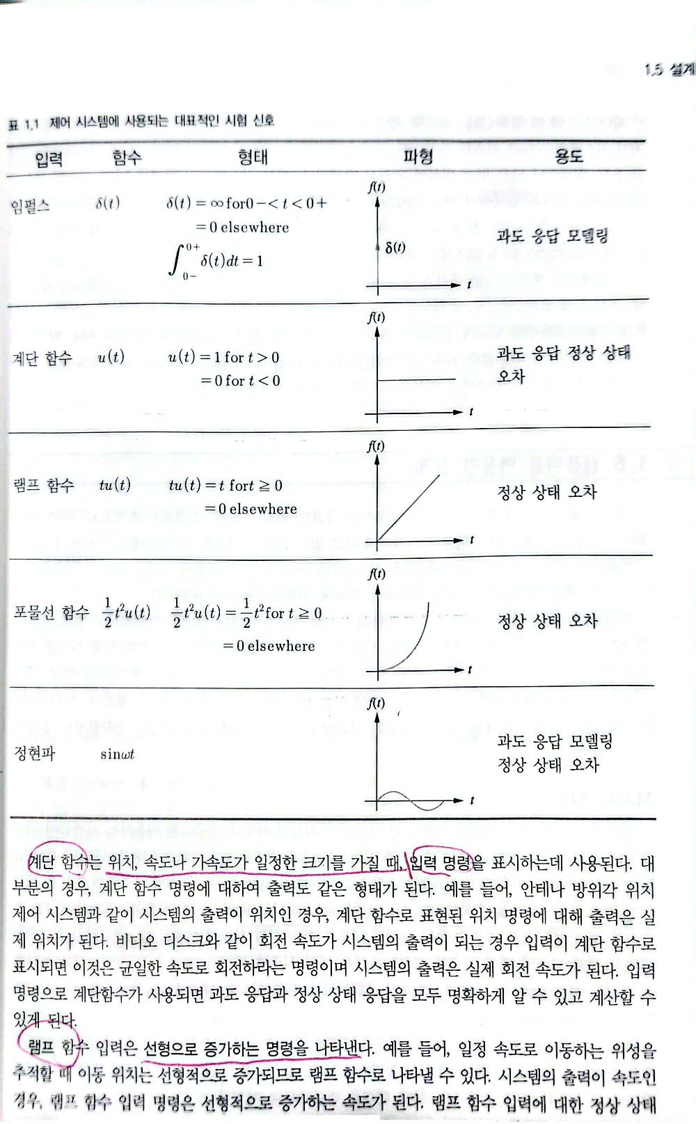
계단 함수 : 위치 속도나 가속도가 일정한 크기를 가질때 입력 명령을 표시하는데 사용됨
램프 함수 입력 : 선형으로 증가하는 명령을 나타냄
정현파 입력 : 시스템에 대한 수학적 모델을 유도하기 위하여 실제 시스템을 시험하는데 이용됨

감도(sensitivity) : 시스템 파라미터 변동에 대한 성능 변동을 퍼센트로

english version

1. System Architecture

1.1 Open-Loop Systems

An open-loop control system operates without feedback.

The system begins with an input transducer, which converts the command into a form suitable for the controller/plant.
The input signal is called the reference input.
The output is referred to as the controlled variable.
Disturbances may enter at a summing junction, where signals are algebraically combined.

Example: A mechanical system composed of a mass, spring, and damper.

A damper dissipates energy (typically proportional to velocity).

Limitation:
Open-loop systems are sensitive to disturbances and cannot automatically correct for unexpected variations, leading to degraded accuracy and robustness.

1.2 Closed-Loop Systems (Feedback Systems)

A closed-loop system uses feedback to reduce error and improve robustness.

The input transducer converts the reference command for the controller.
A sensor (output transducer) measures the output and converts it into a comparable signal form.
The measured output returns through the feedback path to the summing junction.

The error (actuating signal) is:

e(t) = r(t) - y(t)

where:

$r(t)$ : reference input
$y(t)$ : output
$e(t)$ : error (actuating signal)

Compensation

Improving transient response or steady-state error by gain adjustment or controller redesign is called compensation.
The redesigned element is called a compensator.

2. Objectives of Analysis and Design

Control design typically focuses on:

Transient response
Steady-state response
Stability

2.1 Transient Response

Transient response describes system behavior before reaching steady state.

Key measures include:

rise time
peak time
overshoot
settling time

Engineering note: An excessively fast transient can cause actuator saturation or physical damage in real systems.

2.2 Steady-State Response

Steady-state response describes long-term behavior after transients decay.

A key metric is the steady-state error, which depends on:

system type
input class (step, ramp, etc.)

2.3 Stability

If the system is unstable, transient and steady-state specifications are meaningless.

For an LTI system:

\text{Total Response} = \text{Natural Response} + \text{Forced Response}

Natural response = homogeneous solution
Forced response = particular solution

For a stable system:

\lim_{t \to \infty} \text{Natural Response} = 0

Damped Oscillation

A damped oscillation is a transient sinusoidal response whose amplitude decreases over time due to dissipation.

3. Design Procedure

Step 1: Select the Physical System

Select a physical system that satisfies the given performance requirements, constraints, and operating conditions.

Step 2: Build the Functional Block Diagram

Represent each subsystem as a functional block and interconnect them to describe overall signal flow.

Step 3: Draw the Structural Schematic

Example: DC motor drive system

differential amplifier: gain control
power amplifier: power amplification
load: inertia + viscous damping

A common load model:

T = J\dot{\omega} + B\omega

where:

$J$ : inertia
$B$ : viscous damping
$\omega$ : angular velocity

Step 4: Develop the Mathematical Model

Use physical laws:

Kirchhoff’s Voltage/Current Laws (electrical)
Newton’s Second Law (mechanical)

Typical result: an LTI differential equation relating input and output.

Transfer Function

Applying Laplace transform:

G(s) = \frac{Y(s)}{R(s)}

State-Space Model

State equation:

\dot{x} = Ax + Bu

Output equation:

y = Cx + Du

Why state-space?

supports MIMO
handles nonlinear extensions
convenient for simulation
foundation of modern control

Step 5: Block Diagram Reduction

Simplify interconnected blocks using algebraic reduction rules to obtain the overall system form.

Step 6: Analysis and Controller Design

Design the controller to satisfy:

stability
transient performance
steady-state accuracy
robustness

4. Standard Test Inputs

Step input: represents a sudden command (often used in position control evaluation)
Ramp input: represents a linearly increasing command (useful for tracking analysis)
Sinusoidal input: used for frequency-response testing and system identification

5. Sensitivity

Sensitivity measures performance variation due to parameter changes:

S = \frac{\% \text{ change in output}}{\% \text{ change in parameter}}

Low sensitivity implies strong robustness to modeling uncertainty and component tolerances.

6. Core Design Balance

Control design fundamentally balances:

Stability
Performance
Robustness

이준혁

#자기공부 #틀린것도많음 #자기개발 여러분 인생이 힘들다 하더라도 그것을 깨는 순간 큰 희열감으로 옵니다~