Feature Engineering(1) - 피쳐추출

1. 피쳐 엔지니어링

1.1 피쳐

• 데이터 모델에서 예측을 수행하는 변수를 의미한다.
• 통계학에서는 독립변수라고 함
• 피쳐는 속성, 인과관계에 따라 구분할 수 있다.
  - 속성: 범주형, 수치형
  • 인과관계: 독립형, 종속형
• 머신러닝에서는 입력과 출력 변수이냐에 따라서 다르게 불린다.
  - 입력: 변수, 속성, 예측변수, 차원, 관측치, 독립변수
  • 출력: 라벨, 클래스, 목푯값, 반응, 종속변수 등

1.2 피쳐엔지니어링

• 피쳐 엔지니어링은 모형의 성능 개선을 위해 데이터의 지식을 활용하여 변수를 조합하거나 새로운 변수를 만드는 과정
• 피쳐 추출, 피쳐 선택으로 구분할 수 있다.

1.2.1 피쳐 추출(feature extraction)

• 피쳐들 사이에 내재한 특성이나 관계를 분석하여 이들을 잘 표현할 수 있는 새로운 선형 혹은 비선형 결합 변수를 만들어 데이터를 줄이는 방법
• 고차원의 원본 피쳐 공간을 저차원의 새로운 피쳐 공간으로 투영
• PCA(주성분 분석), LDA(선형 판별 분석) 등

1.2.2 피쳐 선택(feature selection)

• 피쳐 중 타겟에 가장 관련성이 높은 피쳐만을 선정하여 피쳐의 수를 줄이는 방법
• 관련없거나 중복되는 피쳐들을 필터링하고 간결한 subset을 생성
• 모델 단순화, 훈련 시간 축소, 차원의 저주 방지, 과적합(Over-fitting)을 줄여 일반화해주는 장점이 있음
• Filter, Wrapper, Embedded 메서드

---

2. 피쳐 추출

2.1 주성분 분석

• 가장 널리 사용되는 차원(변수) 축소 기법 중 하나
• 원 데이터의 분산(variance)을 최대한 보존하면서 서로 직교하는 새 기저(축)를 찾아, 고차원 공간의 표본들을 선형 연관성이 없는 저차원 공간으로 변환하는 기법
• PCA는 기존의 변수를 조합하여 서로 연관성이 없는 새로운 변수, 즉 주성분(principal component, PC)들을 만들어 냄
• 주성분의 개수를 증가시킴에 따라 원 데이터의 분산의 보존수준이 높아짐

from sklearn import datasets
from sklearn.decomposition import PCA
from sklearn.discriminant_analysis import LinearDiscriminantAnalysis`

# iris 데이터셋을 로드
iris = datasets.load_iris()

X = iris.data # iris 데이터셋의 피쳐들
y = iris.target # iris 데이터셋의 타겟
target_names = list(iris.target_names) # iris 데이터셋의 타겟 이름

print(f'{X.shape = }, {y.shape = }') # 150개 데이터, 4 features
print(f'{target_names = }') 

X.shape = (150, 4), y.shape = (150,)
target_names = ['setosa', 'versicolor', 'virginica']

# PCA의 객체를 생성, 차원은 2차원으로 설정(현재는 4차원)
pca = PCA(n_components=2)

# PCA를 수행. PCA는 비지도 학습이므로 y값을 넣지 않음
pca_fitted = pca.fit(X)

print(f'{pca_fitted.components_ = }')  # 주성분 벡터
print(f'{pca_fitted.explained_variance_ratio_ = }') # 주성분 벡터의 설명할 수 있는 분산 비율

X_pca = pca_fitted.transform(X) # 주성분 벡터로 데이터를 변환
print(f'{X_pca.shape = }')  # 4차원 데이터가 2차원 데이터로 변환됨

pcafitted.components = array([[ 0.36138659, -0.08452251, 0.85667061, 0.3582892 ],
[ 0.65658877, 0.73016143, -0.17337266, -0.07548102]])
pcafitted.explained_variance_ratio = array([0.92461872, 0.05306648])
X_pca.shape = (150, 2)

2.2 선형판별분석

• 입력 데이터 세트를 저차원 공간으로 투영(projection)해 차원을 축소하는 기법
• 데이터의 Target값 클래스끼리 최대한 분리할 수 있는 축을 찾음 → 지도 학습
• PCA는 Target값을 사용하지 않으므로 비지도 학습

# PCA의 객체를 생성, 차원은 2차원으로 설정(현재는 4차원)
pca = PCA(n_components=2)

# PCA를 수행. PCA는 비지도 학습이므로 y값을 넣지 않음
pca_fitted = pca.fit(X)

print(f'{pca_fitted.components_ = }')  # 주성분 벡터
print(f'{pca_fitted.explained_variance_ratio_ = }') # 주성분 벡터의 설명할 수 있는 분산 비율

X_pca = pca_fitted.transform(X) # 주성분 벡터로 데이터를 변환
print(f'{X_pca.shape = }')  # 4차원 데이터가 2차원 데이터로 변환됨

ldafitted.coef=array([[ 6.31475846, 12.13931718, -16.94642465, -20.77005459],
[ -1.53119919, -4.37604348, 4.69566531, 3.06258539],
[ -4.78355927, -7.7632737 , 12.25075935, 17.7074692 ]])
ldafitted.explained_variance_ratio=array([0.9912126, 0.0087874])
X_lda.shape = (150, 2)

# 시각화 하기
import matplotlib.pyplot as plt
import seaborn as sns
import pandas as pd

# Seaborn을 이용하기 위해 데이터프레임으로 변환
df_pca = pd.DataFrame(X_pca, columns=['PC1', 'PC2'])
df_lda = pd.DataFrame(X_lda, columns=['LD1', 'LD2'])
y = pd.Series(y).replace({0:'setosa', 1:'versicolor', 2:'virginica'})

# subplot으로 시각화
fig, ax = plt.subplots(1, 2, figsize=(10, 4))

sns.scatterplot(df_pca, x='PC1', y='PC2', hue=y, style=y, ax=ax[0], palette='Set1')
ax[0].set_title('PCA of IRIS dataset')

sns.scatterplot(df_lda, x='LD1', y='LD2', hue=y, style=y, ax=ax[1], palette='Set1')
ax[1].set_title('LDA of IRIS dataset')

plt.show()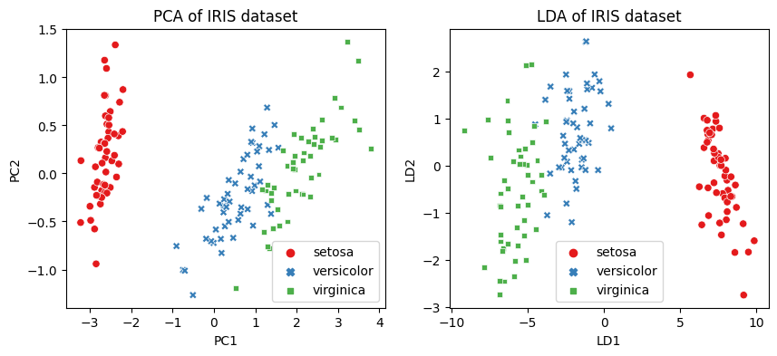

2.3 와인데이터로 PCA와 LDA 연습해보기

2.3.1 PCA 주성분 분석

from sklearn import datasets
from sklearn.decomposition import PCA
from sklearn.discriminant_analysis import LinearDiscriminantAnalysis

# wine 데이터셋을 로드
wine = datasets.load_wine()

X = wine.data  # wine 데이터셋의 피쳐들
y = wine.target  # wine 데이터셋의 타겟
target_names = list(wine.target_names)  # wine 데이터셋의 타겟 이름

# 데이터의 형태 출력
print(f'{X.shape = }, {y.shape = }')  # 데이터는 178개, 13 features
print(f'{target_names = }')  # ['class_0', 'class_1', 'class_2']

X.shape = (178, 13), y.shape = (178,)
target_names = ['class_0', 'class_1', 'class_2']

from sklearn.decomposition import PCA
from sklearn.datasets import load_wine

# wine 데이터셋 로드
wine = load_wine()
X = wine.data

# PCA의 객체를 생성, 차원은 2차원으로 설정(현재는 13차원)
pca = PCA(n_components=2)

# PCA를 수행. PCA는 비지도 학습이므로 y값을 넣지 않음
pca_fitted = pca.fit(X)

print(f'{pca_fitted.components_ = }')  # 주성분 벡터
print(f'{pca_fitted.explained_variance_ratio_ = }')  # 주성분 벡터의 설명할 수 있는 분산 비율

X_pca = pca_fitted.transform(X)  # 주성분 벡터로 데이터를 변환
print(f'{X_pca.shape = }')  # 13차원 데이터가 2차원 데이터로 변환됨

pcafitted.components = array([[ 1.65926472e-03, -6.81015556e-04, 1.94905742e-04,
-4.67130058e-03, 1.78680075e-02, 9.89829680e-04,
1.56728830e-03, -1.23086662e-04, 6.00607792e-04,
2.32714319e-03, 1.71380037e-04, 7.04931645e-04,
9.99822937e-01],
[ 1.20340617e-03, 2.15498184e-03, 4.59369254e-03,
2.64503930e-02, 9.99344186e-01, 8.77962152e-04,
-5.18507284e-05, -1.35447892e-03, 5.00440040e-03,
1.51003530e-02, -7.62673115e-04, -3.49536431e-03,
-1.77738095e-02]])
pcafitted.explained_variance_ratio = array([0.99809123, 0.00173592])
X_pca.shape = (178, 2)

2.3.2 LDA 선형판별분석

# LDA의 객체를 생성. 차원은 2차원으로 설정(현재는 13차원)
lda = LinearDiscriminantAnalysis(n_components=2)

# LDA를 수행. LDA는 지도학습이므로 타겟값이 필요
lda_fitted = lda.fit(X, y)

print(f'{lda_fitted.coef_=}')  # LDA의 계수
print(f'{lda_fitted.explained_variance_ratio_=}')  # LDA의 분산에 대한 설명력

X_lda = lda_fitted.transform(X)
print(f'{X_lda.shape = }')  # 13차원 데이터가 2차원 데이터로 변환됨

ldafitted.coef=array([[ 2.85542117e+00, -4.89788666e-02, 5.23156990e+00,
-7.77422596e-01, 6.62170776e-03, -2.16976970e+00,
4.85310738e+00, 2.36037857e+00, -9.78422688e-01,
-7.86790206e-01, 2.35758911e-01, 4.04832027e+00,
1.40369442e-02],
[-2.12348259e+00, -7.68274072e-01, -5.77105386e+00,
3.49607787e-01, 1.31672488e-03, 3.03762476e-02,
1.34898232e+00, 4.15204322e+00, 7.48631160e-01,
-6.54459561e-01, 3.81286126e+00, -3.42724866e-02,
-6.83988909e-03],
[-3.68803859e-01, 1.19660859e+00, 2.10587916e+00,
4.38453756e-01, -1.00868380e-02, 2.62207706e+00,
-7.96064750e+00, -9.04286258e+00, 9.52942959e-02,
1.93515106e+00, -5.92964428e+00, -4.92536562e+00,
-7.13640797e-03]])
ldafitted.explained_variance_ratio=array([0.68747889, 0.31252111])
X_lda.shape = (178, 2)

import matplotlib.pyplot as plt
import seaborn as sns
import pandas as pd
from sklearn.decomposition import PCA
from sklearn.discriminant_analysis import LinearDiscriminantAnalysis

# PCA 수행
pca = PCA(n_components=2)
X_pca = pca.fit_transform(X)

# LDA 수행
lda = LinearDiscriminantAnalysis(n_components=2)
X_lda = lda.fit_transform(X, y)

# Seaborn을 이용하기 위해 데이터프레임으로 변환
df_pca = pd.DataFrame(X_pca, columns=['PC1', 'PC2'])
df_lda = pd.DataFrame(X_lda, columns=['LD1', 'LD2'])
y = pd.Series(y).replace({0: 'class_0', 1: 'class_1', 2: 'class_2'})

# subplot으로 시각화
fig, ax = plt.subplots(1, 2, figsize=(10, 4))

# PCA 시각화
sns.scatterplot(data=df_pca, x='PC1', y='PC2', hue=y, style=y, ax=ax[0], palette='Set1')
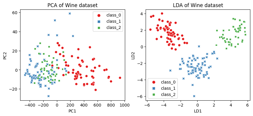
ax[0].set_title('PCA of Wine dataset')

# LDA 시각화
sns.scatterplot(data=df_lda, x='LD1', y='LD2', hue=y, style=y, ax=ax[1], palette='Set1')
ax[1].set_title('LDA of Wine dataset')

plt.show()