<Course Outline>

1. Traditional Feature-based Methods: Node
2. Traditional Feature-based Methods: Link
3. Traditional Feature-based Methods: Graph

2.1 - Traditional Feature-based Methods: Node

Traditional ML Pipline

: is about designing proper features!

• Traditional ML : hand-designed features 을 이용
• Design features for nodes/links/graphs ⇒ 효과적인 feature representation 을 찾는 것이 performance ↑
  1. structural feature(ex. positional...) → Graph-level prediction
  2. attributes and properties of node → Node / Link level prediction

Machine Learning in Graphs

• Goal: Make predictions for a set of objects
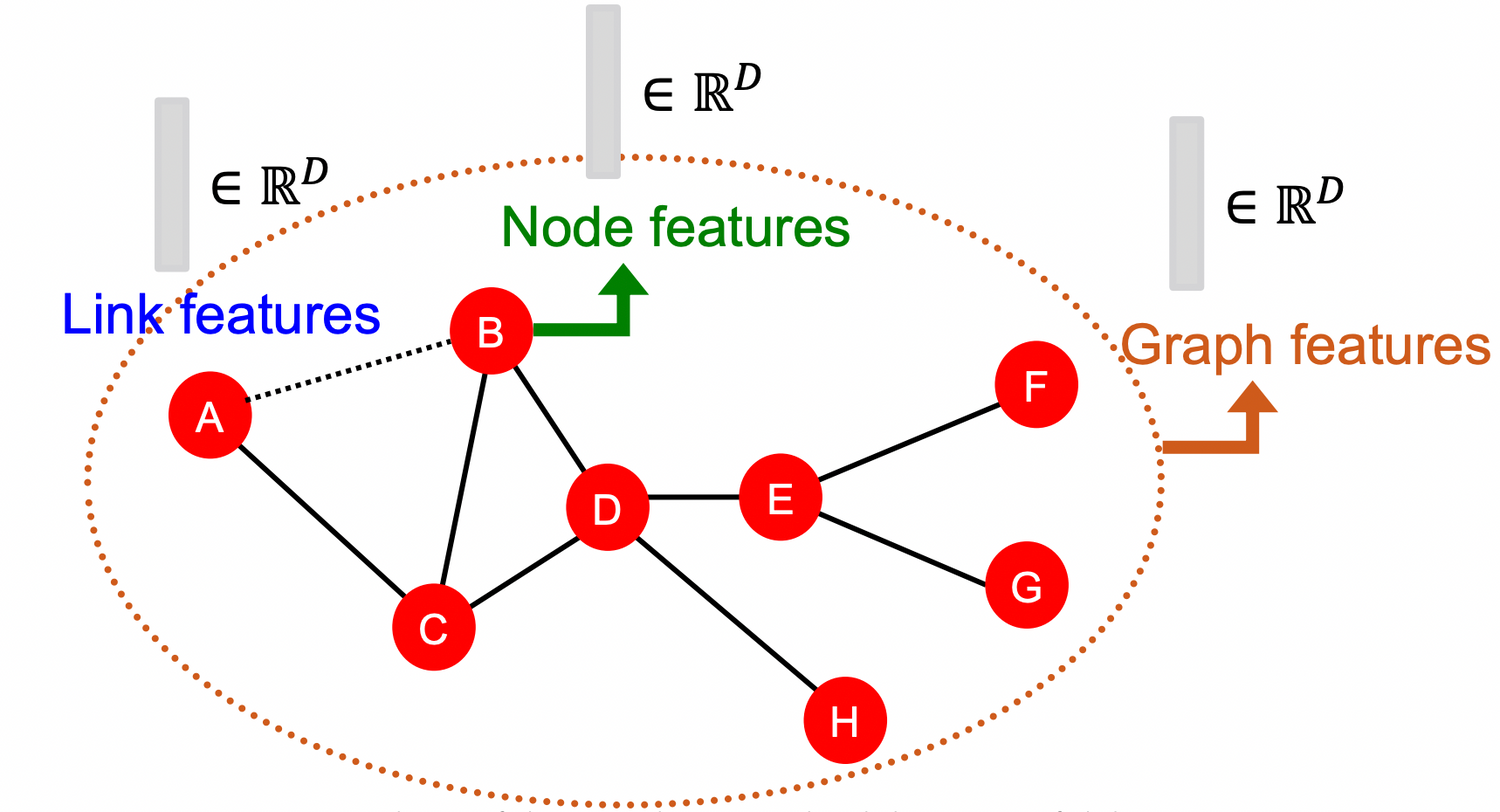
• Design choices:
  • Features : d-dimensional vectors
  • Objects : Nodes, edges, sets of nodes, entire graphs
  • Objective function : What task are we aiming to solve? (풀고자 하는 문제에 따라 다름)

💡 Given : $G = (V,E)$ ⇒ learn a fuction $f : V → \mathbb{R}$

Node-level Tasks and Features

Goal: Characterize the structure and position of a node in the network using

1. Node degree
2. Node centrality
3. Clustering coefficient
4. Graphlets

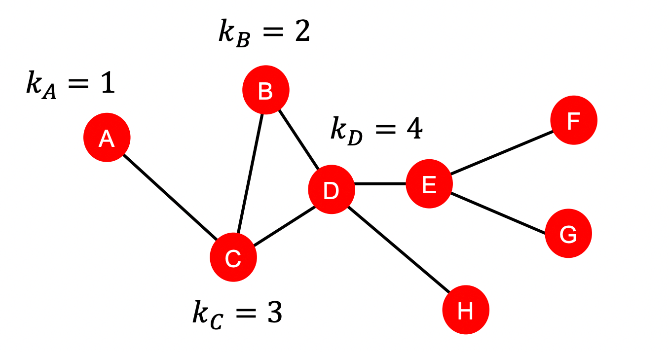
1) Node degree

degree $k_v$ : the node $v$ 가 가진 edge ( = neighboring nodes) 의 수

• 모든 이웃 노드를 동일하게 취급 → 이웃 노드의 importance를 capture 할 수 없음
• 한계) 해당 feature만 사용하면, 모델이 같은 차수를 갖는 노드를 모두 똑같이 예측할 것임

2) Node Centrality

: 노드 $v$ 의 이웃 노드의 centrality의 합이 크면 importance ↑

Node Centrality $c_v$ : 그래프에서 노드가 얼마나 중요한지 고려

• Different ways to model importance
  1. Eigenvector centrality
  2. Betweenness centrality
  3. Closeness centrality
  4. and many others…

Eigenvector centrality

Q) 여기서 centrality는 무엇인가(어떤 값인가)? 결정되지 않은 값인가?
A) Eigenvalue-eigenvector 방정식을 푼다 = 고유값 분해를 통해서 고유값 $\lambda$ 와 고유벡터 $v$를 동시에 구해야하는 연립방정식인 “eigenvalue problem”을 해결하는 것이므로 → $\lambda$ 와 $v$ 가 동시에 결정됨.

centrality of node $v$ = the sum of the centrality of neighboring nodes

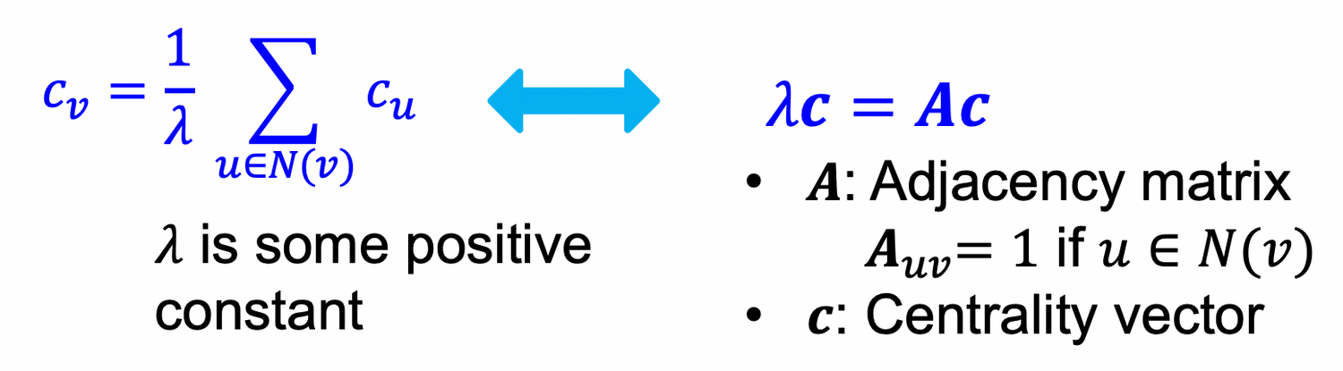
c : eigenvector ⇒ leading eigenvector $c_{max}$ : used for centrality

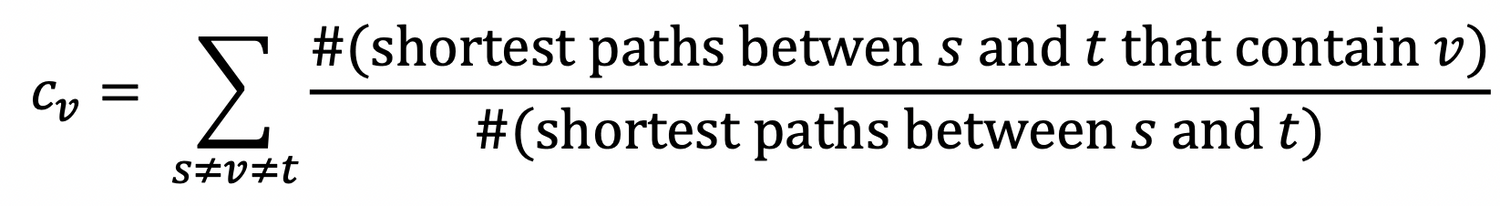
Betweenness centrality

: 임의의 노드 $s$ → $t$ 로 가는 최단 경로에 노드 $v$가 속한 경로가 많을수록 importance ↑

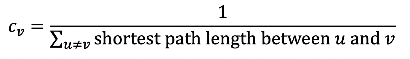
Closeness centrality

: 다른 모든 노드 $u$ 에서 → $v$ 로 가는 최단 경로가 짧을 수록 importance ↑

= 가장자리에 위치한 노드일수록 다른 노드로부터 거리가 멀어짐 ↑

3) Clustering Coefficient

: measures node degree & local structure around the nodes

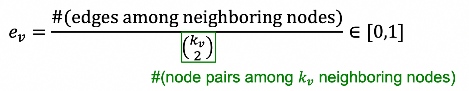
→ 연결 가능한 노드 중에서 실제로 몇개가 연결되어 있는가?

0 : 하나도 연결 X , 1 : 연결 가능한 모든 노드를 연결

Example )

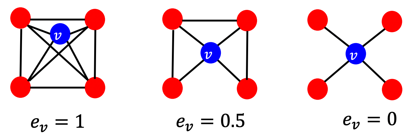
: $e_v = {6 \over {_{4}C_{2}} }$ = 1 ⇒ $k_v$ = 4 (빨간색 노드=이웃노드 개수) , 이웃노드는 총 6개의 엣지로 서로 연결되어 있음

💡 Observation : Clustering coefficient counts the #(triangles) in the ego-network

ego-network = 노드 $v$ 와 그 주변 노드를 의미 = neighborhood network around a given node

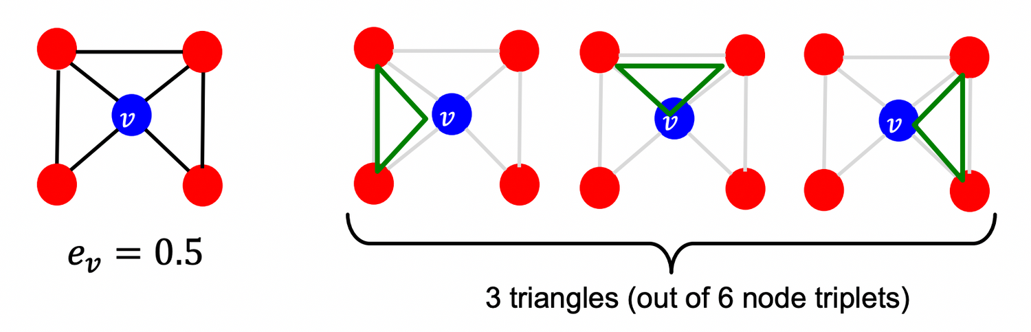
$e_v = \frac{3} {6} = 0.5$ , 3 = # of triangle

→ We can generalize the above by counting #(pre-specified subgraphs, i.e., graphlets).

4) Graphlets

Rooted connected non-isomorphic subgraphs:

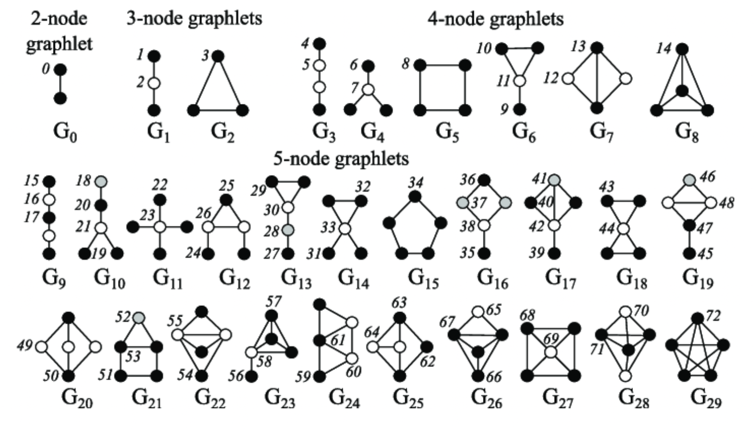
+) 3-node graphlets에서 1번 노드 =/= 2번 노드 지만, 1번 노드는 2번 아래에 있는 노드와는 (회전하면) 같은 노드로 볼 수 있다. → 1번과 2번은 non-isomorphic , 1번과 2번 아래의 노드는 isomorphic 하다고 할 수 있다.

Graphlet Degree Vector (GDV)

: A count vector of graphlets rooted at a given node

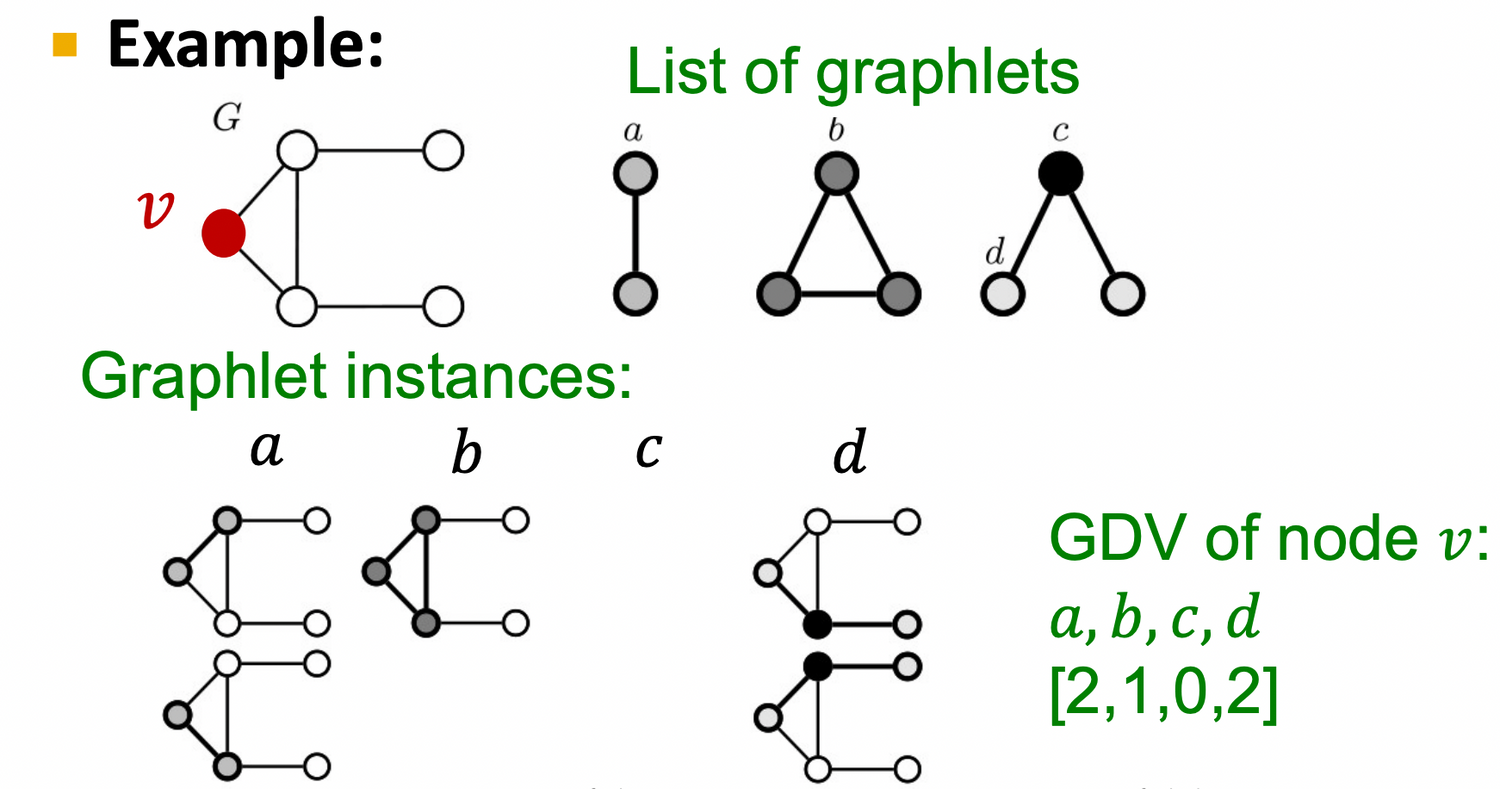
Considering graphlets on 2 to 5 (노드 2개짜리 ~ 5개짜리 graphlet) nodes we get :

• Vector of 73 coordinates is a signature of a node that describes the topology of node's neighborhood → 총 73개의 서로 다른 graphlet이 존재할 수 있음 → graphlet이 노드 이웃의 위상 구조 설명
• Captures its interconnectivities out to a distance of 4 hops → 5개짜리 graphlet은 노드 $v$로부터 4hop 떨어진 (length = 4) path가 몇개 있는지 count하는 것!
• 두개 노드를 가지고 비교하는 node degrees or clustering coefficient 보다 더 자세한 local topological similarity를 측정 가능!

< Summary >

• Degree : counts #(edges) that a node touches
• Clustering coefficient : counts #(triangles) that a node touches.
• GDV : counts #(graphlets) that a node touches

2.2 - Traditional Feature-based Methods: Link

Link-Level Prediction Task

= 존재하는 link에 기반하여 새로운 link를 예측하는 task

• At test time : 존재하는 link를 제외한 모든 노드 pair를 rank → Top K개의 node쌍에서 link가 발생할 것이라고 예측
• key 🔑 : design features for a pair nodes !

단순히 노드 pair의 feature를 concat해서 train하는 방법은 좋지 X → 두 노드 사이 관계에서 중요한 정보를 잃을 수 있음.

Two formulations of the link prediction task:

1. Links missing at random: 랜덤하게 제거한 링크를 예측
   • Remove a random set of links and then aim to predict them
   • static network 예측에 유리
     • ex) protein-protein interaction network
2. Links over time: 시간에 따라 예측
   • Given : $G[t_0,t’_0]$ a graph on edges up to time $t’_0$ ($t_0$ 와 $t’_0$ 사이에 발생한 노드)
   • output : a ranked list L of links (not in $G[t_0,t’_0]$) that are predicted to appear in $G[t_1,t’_1]$ (다음 step $t_1$ ~ $t’_1$ 에 발생할 노드의 랭킹을 예측)
   • Evaluation (학습 방법) :
     • $n = |E_{new}|$ : # new edges that appear during the test period $[t_1,t’_1]$
     • L에서 top n 개의 edge를 예측 → 실제로 발생한 edge와 비교하여 count correct edges
   • 시간에 따라 evolve하는 네트워크 예측에 유리
     • ex) social media network, citation network ...

Link-Level Features

1) Distance-based feature

= 두 노드 사이의 최단 경로를 feature로 사용

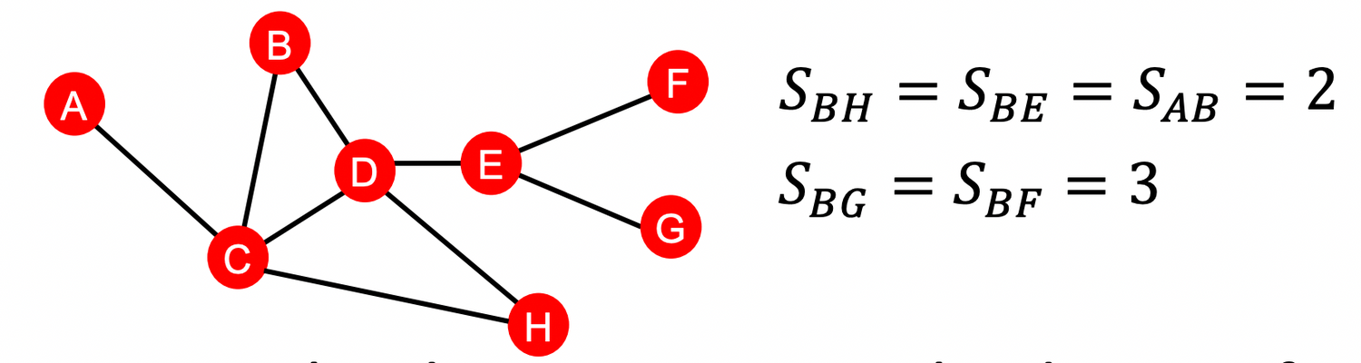
한계 ) 두 노드 사이의 distance는 체크할 수 있지만, degree of neighborhood overlap 은 capture X :

• 예를 들어, Node pair (B, H) 는 B→ D → H , B → C → H 두 종류의 최단경로를 가짐
• pairs (B, E) and (A, B) 같은 경우에는 1 개의 최단경로를 가짐
• 하지만 이 둘을 똑같이 취급함. ⇒ Strength of connection를 capture하기 위해서 2)가 등장

2) Local neighborhood overlap

= 두 노드의 공통된 이웃을 계산

1. Common neighbors:

   $| N(v_1)∩ N(v_2) |$

2. Jaccard’s coefficient:

   $\frac {| N(v_1) ∩ N(v_2)| }{|N(v_1)∪N(v_2)| }$
   • |N(v_1)∪N(v_2)| 가 normalize하는 역할을 했을 뿐, 개념은 1)과 같음.

3. Adamic-Adar index:

   $\sum_{u∈N(v_1)∩N(v_2)} \frac{1}{log(k_u)}$
   • practically used
   • $k_u$ : degree of node $u$
   • 엣지가 많은 노드보다, 엣지가 적은 노드와 연결되었을 때 더 큰 점수를 부여

   한계 ) 공통된 이웃이 없을 경우 항상 0을 출력 → 2hop보다 멀리 떨어진 노드는 항상 0!

   ⇒ 이러한 한계를 보완하기 위해 3)이 등장

3) Global neighborhood overlap

Katz index : count the number of paths of all lengths between two nodes.

💡 How to compute #paths between two nodes?
⇒ Use powers of the graph adjacency matrix!

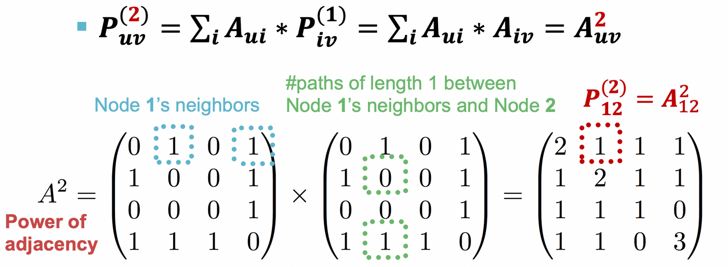
$A_{uv}$ specifies #paths of length 1 (direct neighborhood) between $u$ and $v$.

& $A_{uv}^l$ specifies #paths of length $l$.

Proof ) How to compute $P_{uv}^{(2)}$ ?

노드 u와 v가 2-hop만큼 떨어진 path를 가지기 위해서는

→ u로부터 1의 path를 가지는 임의의 노드 i 가 존재해야함 * 다시 i로부터 v로 가는 path가 존재해야 함.

둘중에 하나라도 존재하지 않으면 곱셈했을 때 0이 나오게 된다.

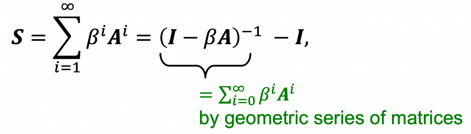
⇒ Katz index between $v_1$ and $v_2$ is calculated as

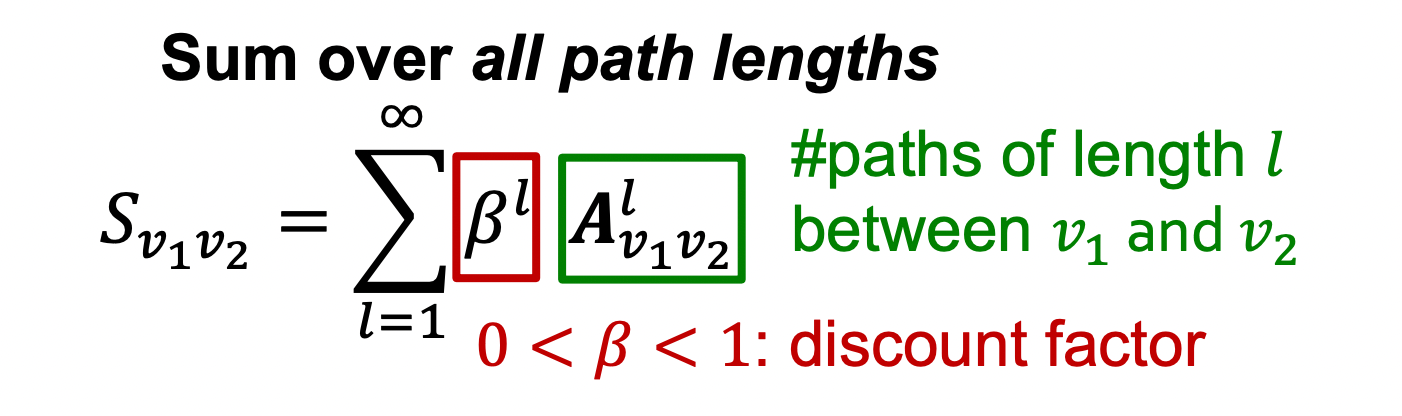
• discount factor $\beta$ = length에 따라 exponentially 감소하면서 longer path에 더 낮은 importance를 부여하게 된다.
• Katz index matrix is computed in closed-form:
  

2.3 - Traditional Feature-based Methods: Graph

How do we create feature vectors from graphs in a sccalable & interesting way?

• Goal: We want features that characterize the structure of an entire graph.
  전체 그래프 구조의 특성을 반영할 수 있는 feature 표현을 찾는 것.

Background : Kernel Methods

Idea : feature vector 를 디자인X ⇒ Kernel 을 디자인 O

A quick introduction to Kernels:

• Kernel $K(G,G') ∈ ℝ$ : measures similarity b/w two graphs

• Kernel matrix $K = (K(G,G'))_{G,G'}$must always be positive semidefinite
  (i.e., has positive eigenvals)

• There exists a feature representation $\phi(•)$ such that $K(G,G') = \phi(G)^T\phi(G')$

• kernel을 사용했을 때 👍 : doesn’t even need to be explicitly created for us to be able to compute the value of the kernel → Once the kernel is defined, off-the-shelf ML model, such as kernel SVM, can be used to make predictions. (커널이 정의되면 커널 SVM과 같은 기성 ML 모델을 사용하여 예측할 수 있습니다.)

Graph Kernels

• Goal: Design graph feature vector $\phi(G)$
• Key idea: Bag-of-Words (BoW) for a graph
  • Both Graphlet Kernel and Weisfeiler-Lehman(WL) Kernel use Bag-of-* representation of graph.

종류

1. Graphlet Kernel [1] : Bag-of-graphlets
2. Weisfeiler-Lehman Kernel [2] : Bag-of-colors
3. Other kernels are also proposed in the literature (beyond the scope of this lecture)
   • Random-walk kernel
   • Shortest-path graph kernel
   • And many more…

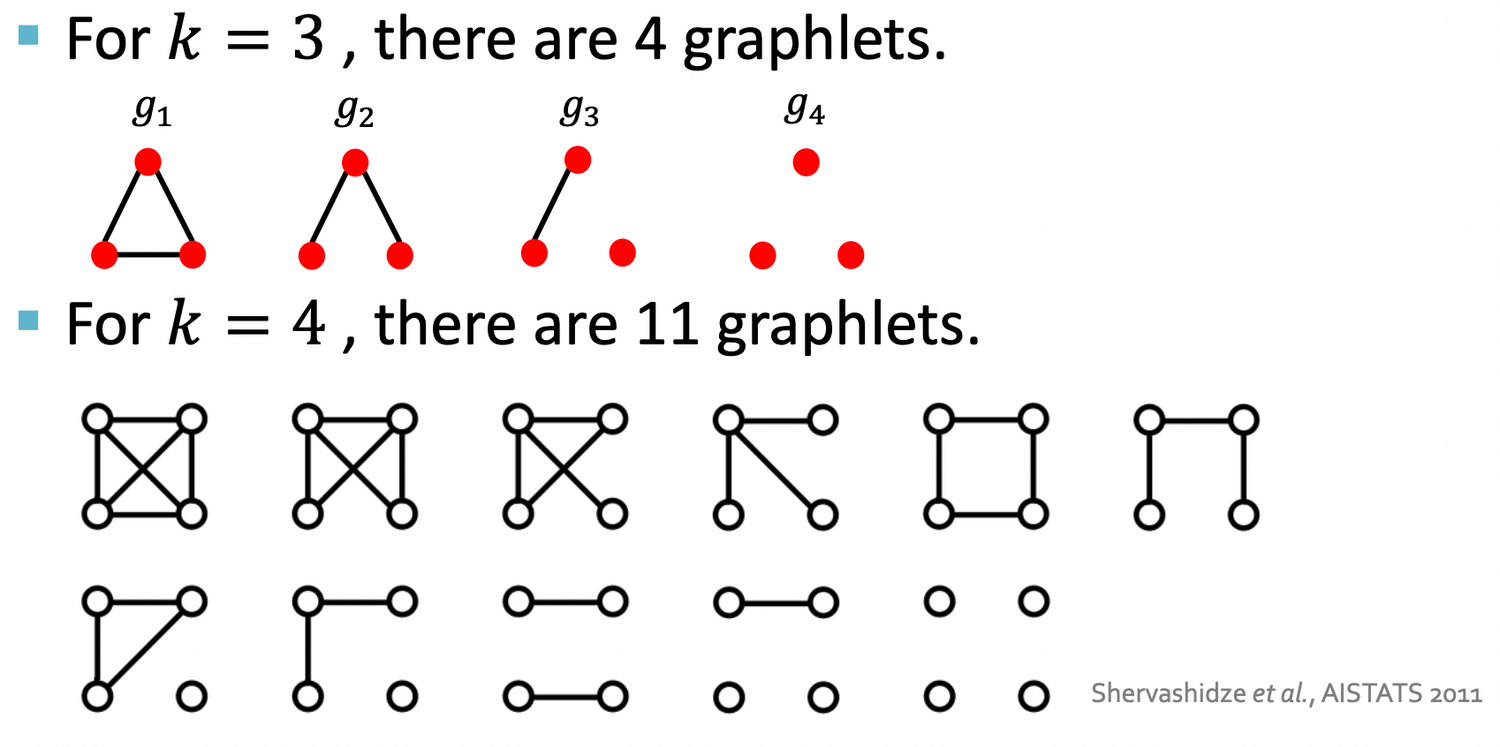
1) Graphlet Features

• Key idea: Count the number of different graphlets in a graph. 💡 Note: node-level features에서 배운 graphlets 정의와 다르다 !
  • The two differences are: graplhet이 connected & rooted 되어 있지 않다

Definite of graphlet in graphlet kernel

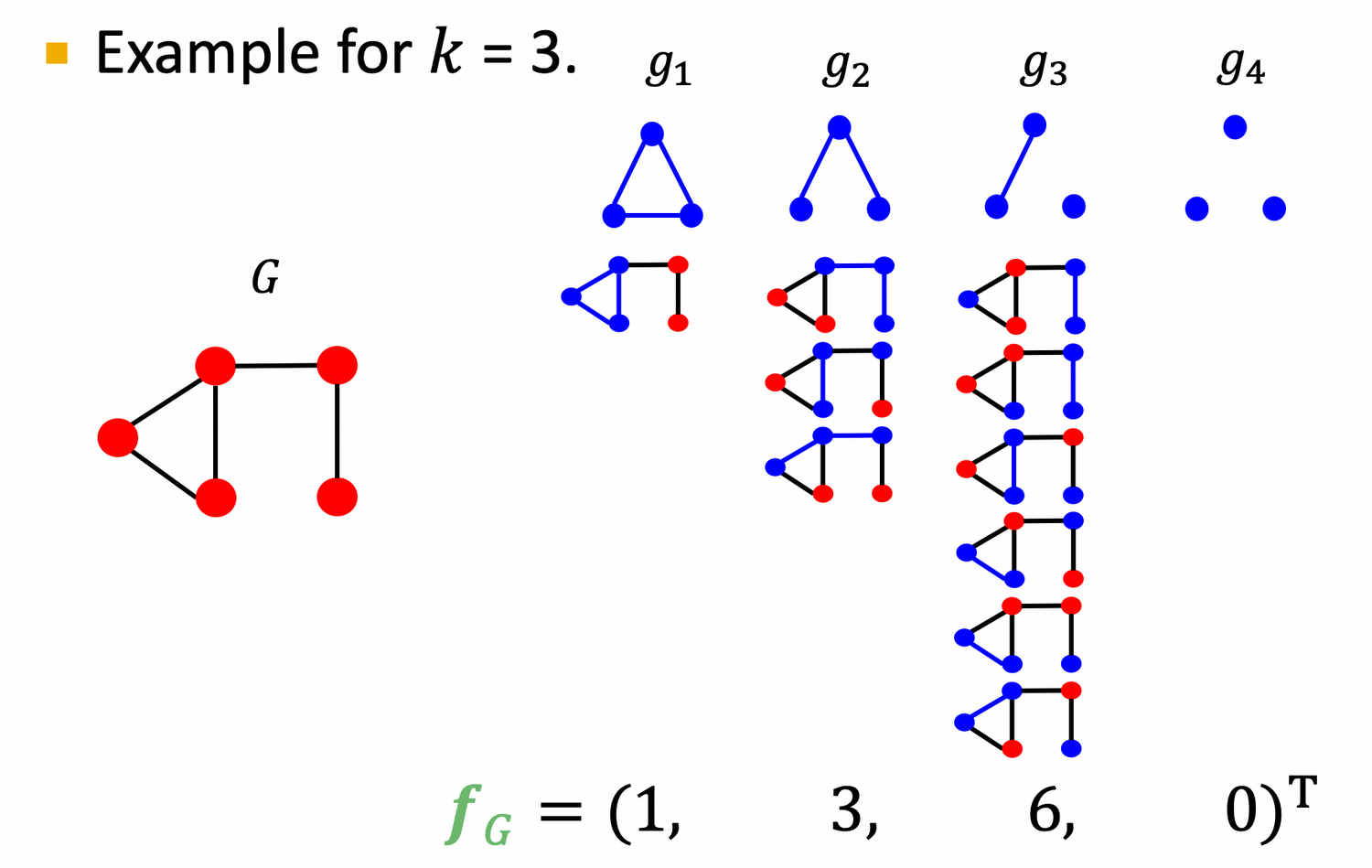
: Let $\mathcal{G_k} = (g_1, g_2, … , g_{n_k})$ be a list of graphlets of size $k$

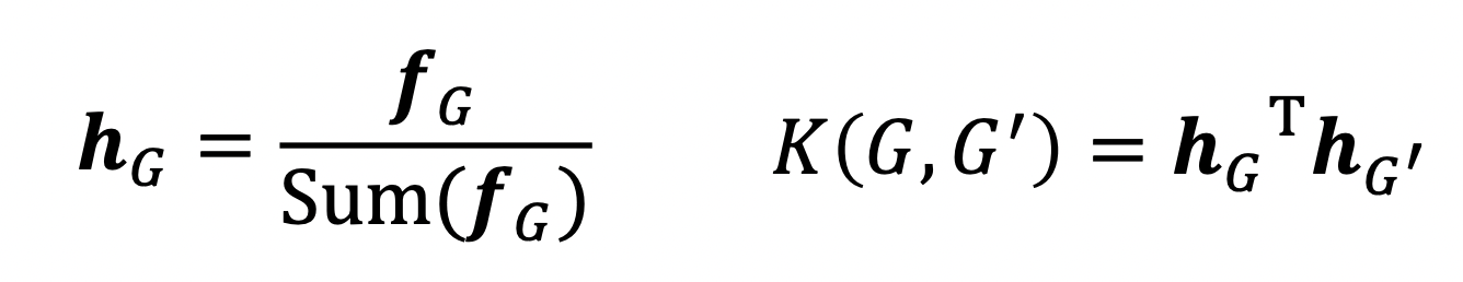
Given graph $G$, and a graphlet list $\mathcal{G_k} = (g_1, g_2, … , g_{n_k})$, define the graphlet count vector $f_G ∈ ℝ^{n_k}$ as

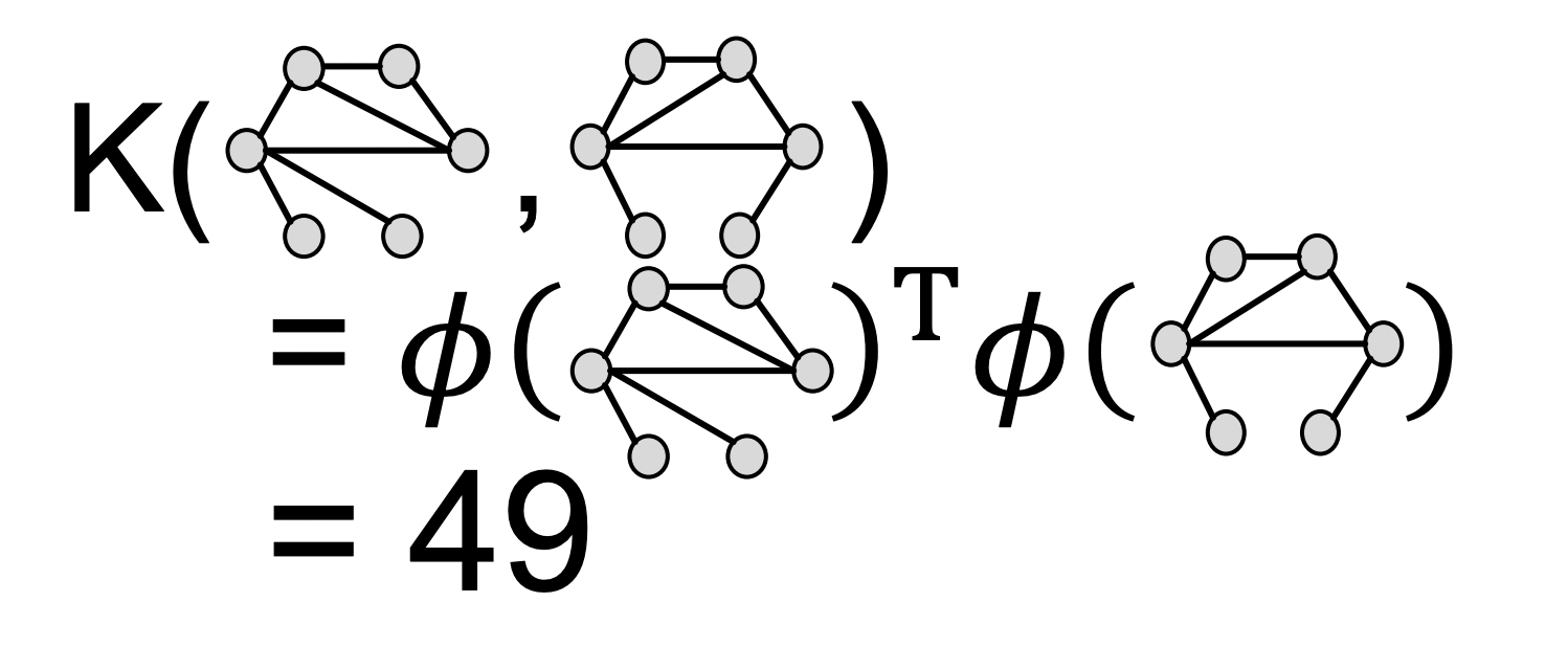
Given two graphs, $G$ and $G’$ , graphlet kernel is computed as

• Problem: if G and G’ have different sizes, that will greatly skew the value.
• Solution: normalize each feature vector
  
• Limitations : Counting graphlets is expensive!
  • 논문읽기

🥺 how can we design more efficeint kernel? ⇒ W-L Kernel

2) Weisfeiler-Lehman Kernel

• Goal: design an efficient graph feature descriptor $\phi(G)$
• idea: use neighborhood structure to iteratively enrich node vocabulary.
  • Bag of node degrees를 one-hop ~ multi-hop으로 일반화 한 것!
  • Algorithm to achieve this: Color Refinement

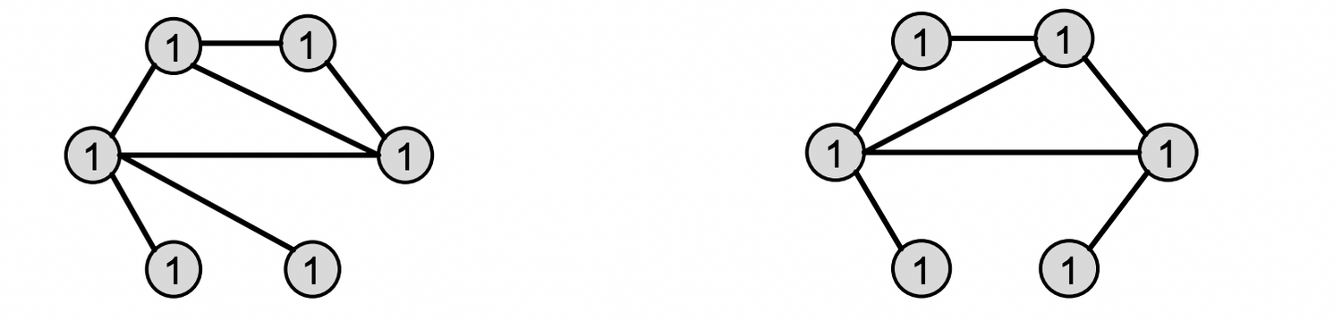
Example of color refinement given two graphs

Given : A graph $G$ with a set of nodes $v$

1. Assign an initial color $c^{(0)}(v)$ to each node $v$. : 모두 같은 색으로 초기화

   

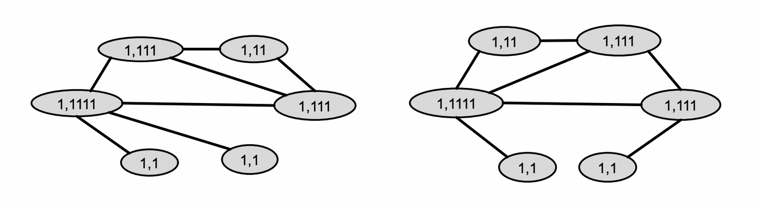
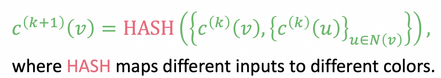
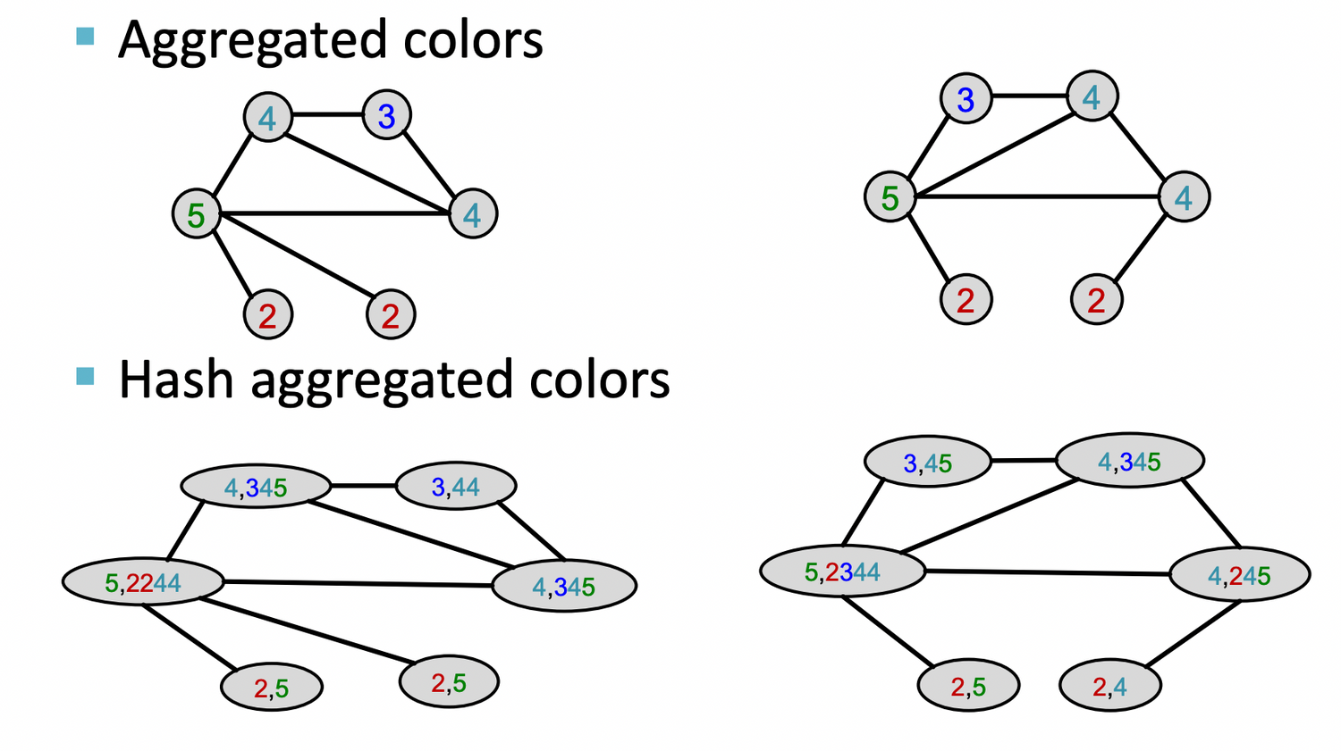
2. Aggregate neighboring colors

   

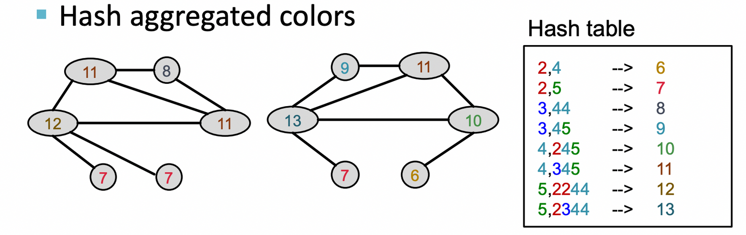
3. Hash aggregated colors
   
   

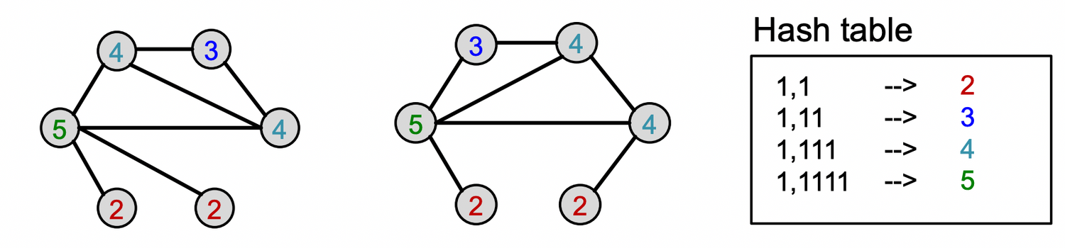
4. 이를 K번 반복 (여기서는 K=3)
   
   

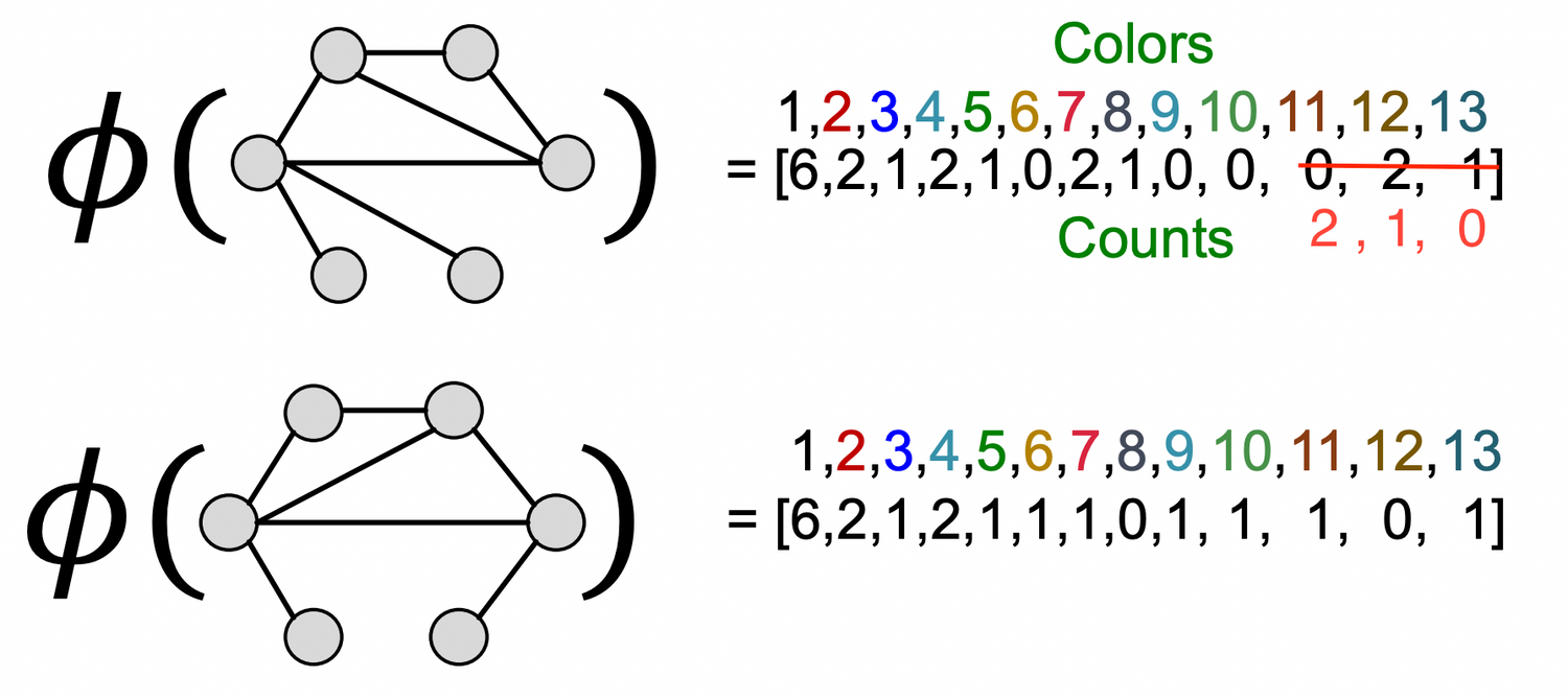
5. After K steps of color refinement, WL kernel counts number of nodes with a given color.

   

   : $c^{(K)}(v)$ summarizes the structure of K-hop neighborhood

6. The WL kernel value is computed by the inner product of the color count vectors:

   

WL kernel is computationally efficient.

• 각 step에서 이웃의 color를 집계하는데 필요한 time complexity : linear in #(edges)
  • 각 노드에서 이어진 모든 엣지를 따라 집계 + hashfunc. 적용 하기만 하면 됨
• kernel value 를 계산하기 위해서 두 그래프에 나타난 색깔이 tracked될 필요가 있는데
  • 색깔의 개수는 노드 개수를 넘지 않으므로 #(colors) ≤ #(nodes)
  • Counting colors : linear-time of #(nodes)

⇒ In total, time complexity is linear in #(edges).

cf> Closely related to Graph Neural Networks (as we will see!)