[Tensorflow] 1. TensorFlow for Artificial Intelligence, Machine Learning, and Deep Learning Paradigm(3 week Enhancing Vision with Convolutional Neural Networks) - programming (2)

[Tensorflow] 1. TensorFlow for Artificial Intelligence, Machine Learning, and Deep Learning Paradigm(3 week Enhancing Vision with Convolutional Neural Networks) - programming (2)

Exploring Convolutions / Max pooling

[1] input data setting & Library import

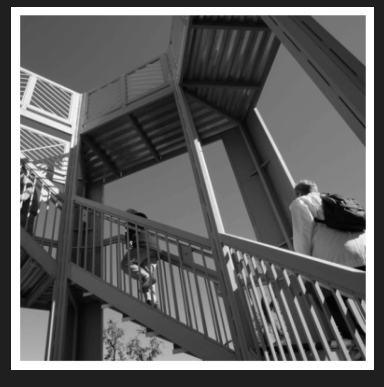
Scipy에서 misc 라이브러리를 임포트한다.
misc.ascent를 이미지를 사용하기 쉽게 반환해서 직접 조정할 필요가 없다.

from sicpy import misc

ascent_image = misc.ascent()

matplotlib은 이미지를 그리는 코드를 가지고 있다.

import matplotlib.pyplot as plt

plt.grid(False)
plt.gray()
plt.axis('off')
plt.imshow(ascent_image)
plt.show()

scipy에서 불러온 올라가는 이미지를 볼 수 있다.

**[2] Add Convolution

그 이후 직접 만든 컨볼루션과 함께 추가한 다음
이미지의 x 및 y 사이즈를 추적하는 변수를 생성한다.
여기 이미지의 사이즈는 512 * 512이다.

import numpy as np

image_transformed = np.copy(ascent_image)

size_x = image_transformed.shape[0]
size_y = image_transformed.shape[1]

print(size_x, size_y)

3x3 배열로 컨볼루션을 만든다.
날카로운 모서리를 감지하기 좋은 값을 불러온다.

filter = [[0,1,0],[1,-4,1],[0,1,0]]

weight = 1

해당 코드가 바로 컨볼루션을 생성하는데,
이미지를 반복하면서 1픽셀의 마진을 준다.

# Iterate over the image
for x in range(1,size_x-1):
 for y in range(1,size_y-1):
     convolution = 0.0
     convolution = convolution + (ascent_image[x-1, y-1] * filter[0][0])
     convolution = convolution + (ascent_image[x-1, y] * filter[0][1])  
     convolution = convolution + (ascent_image[x-1, y+1] * filter[0][2])     
     convolution = convolution + (ascent_image[x, y-1] * filter[1][0])    
     convolution = convolution + (ascent_image[x, y] * filter[1][1])    
     convolution = convolution + (ascent_image[x, y+1] * filter[1][2])    
     convolution = convolution + (ascent_image[x+1, y-1] * filter[2][0])    
     convolution = convolution + (ascent_image[x+1, y] * filter[2][1])    
     convolution = convolution + (ascent_image[x+1, y+1] * filter[2][2])    
     
     # Multiply by weight
     convolution = convolution * weight   
     
     # Check the boundaries of the pixel values
     if(convolution<0):
       convolution=0
     if(convolution>255):
       convolution=255

     # Load into the transformed image
     image_transformed[x, y] = convolution

루프가 0이 아닌 1부터 시작하고 x-1, y-1 사이즈에서 끝난다.
루프 내에서 컨볼루션을 계산한다.
픽셀과 그 이웃을 확인하고 필터로 결정된 값으로 이들 값을 곱한 다음, 마지막으로 전부 더하는 것이다.

# Plot the image. Note the size of the axes -- they are 512 by 512
plt.gray()
plt.grid(False)
plt.imshow(image_transformed)
plt.show()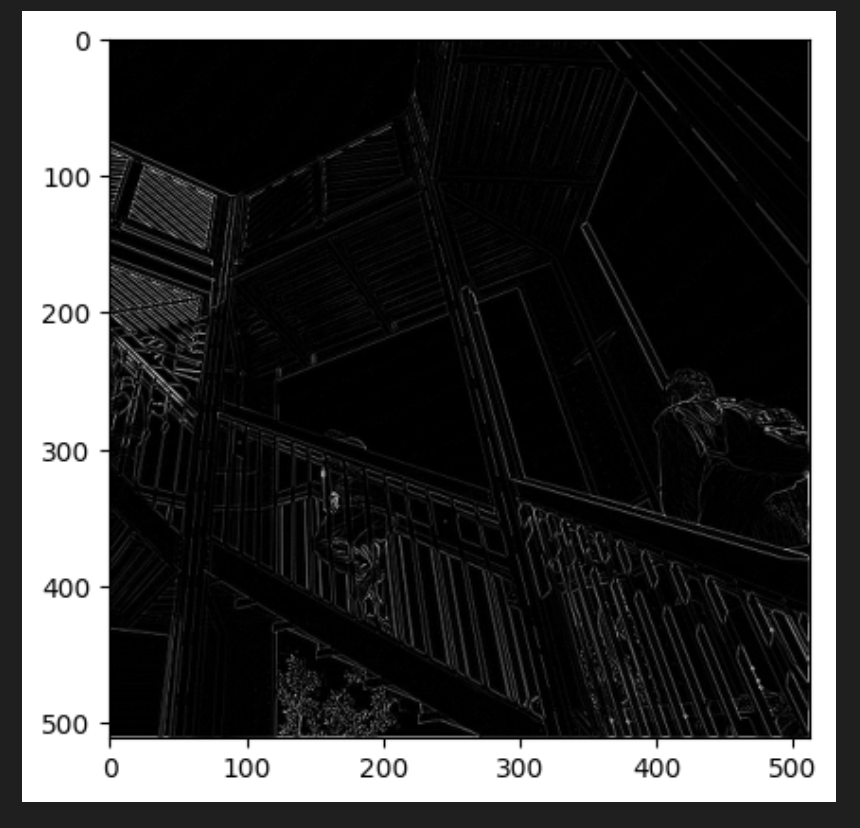   

결과를 보면 일부 특징만 필터를 통과한 것을 볼 수 있다.
두 어개의 필터를 추가로 수정해서 확인해볼 수 있다.

다음은 수직선 자리를 포착하기 좋은 필터이다.

filter = [ [-1, -2, -1], [0, 0, 0], [1, 2, 1]]

weigth = 1
for x in range(1,size_x-1):
  for y in range(1,size_y-1):
      convolution = 0.0
      convolution = convolution + (ascent_image[x-1, y-1] * filter[0][0])
      convolution = convolution + (ascent_image[x-1, y] * filter[0][1])  
      convolution = convolution + (ascent_image[x-1, y+1] * filter[0][2])     
      convolution = convolution + (ascent_image[x, y-1] * filter[1][0])    
      convolution = convolution + (ascent_image[x, y] * filter[1][1])    
      convolution = convolution + (ascent_image[x, y+1] * filter[1][2])    
      convolution = convolution + (ascent_image[x+1, y-1] * filter[2][0])    
      convolution = convolution + (ascent_image[x+1, y] * filter[2][1])    
      convolution = convolution + (ascent_image[x+1, y+1] * filter[2][2])    
      
      # Multiply by weight
      convolution = convolution * weight   
      
      # Check the boundaries of the pixel values
      if(convolution<0):
        convolution=0
      if(convolution>255):
        convolution=255

      # Load into the transformed image
      image_transformed[x, y] = convolution
      
plt.gray()
plt.grid(False)
plt.imshow(image_transformed)
plt.show()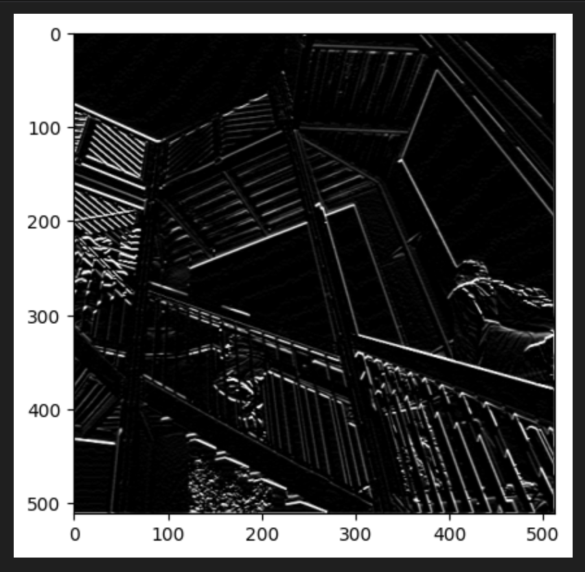   

실행후에 플랫을 보면 이미지의 수직선이 표시된 것을 볼 수 있다.
단지 상하 직선이 아니라 이미지 자체의 관점에서 봤을 때 수직이라는 점이다.

다음 필터는 수평선을 표시하는 것이다.

filter = [ [-1, 0, 1], [-2, 0, 2], [-1, 0, 1]]

weigth = 1
for x in range(1,size_x-1):
  for y in range(1,size_y-1):
      convolution = 0.0
      convolution = convolution + (ascent_image[x-1, y-1] * filter[0][0])
      convolution = convolution + (ascent_image[x-1, y] * filter[0][1])  
      convolution = convolution + (ascent_image[x-1, y+1] * filter[0][2])     
      convolution = convolution + (ascent_image[x, y-1] * filter[1][0])    
      convolution = convolution + (ascent_image[x, y] * filter[1][1])    
      convolution = convolution + (ascent_image[x, y+1] * filter[1][2])    
      convolution = convolution + (ascent_image[x+1, y-1] * filter[2][0])    
      convolution = convolution + (ascent_image[x+1, y] * filter[2][1])    
      convolution = convolution + (ascent_image[x+1, y+1] * filter[2][2])    
      
      # Multiply by weight
      convolution = convolution * weight   
      
      # Check the boundaries of the pixel values
      if(convolution<0):
        convolution=0
      if(convolution>255):
        convolution=255

      # Load into the transformed image
      image_transformed[x, y] = convolution
      
plt.gray()
plt.grid(False)
plt.imshow(image_transformed)
plt.show()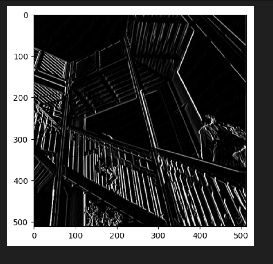   

필터를 실행하고 플롯을 구성하면 수평선 여러 개가 생겨난 것을 볼 수 있다.

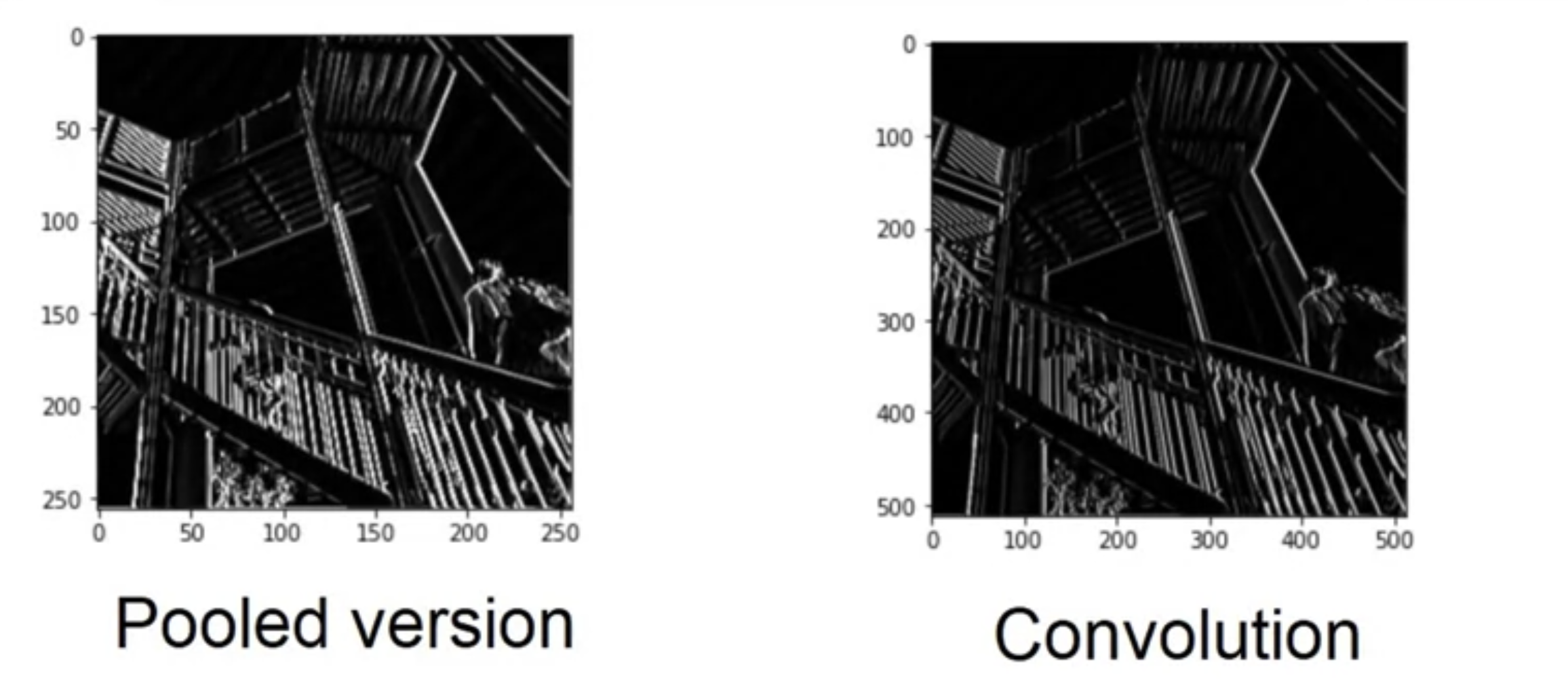
Max Pooling

맥스 풀링은 4개의 청크로 이루어진 픽셀만 취해서 가장 큰 값만 통과시킨다.
코드를 실행하고 출력값을 렌더링해보자.

new_x = int(size_x/2)
new_y = int(size_y/2)

print(new_x)
print(new_y)

#output
256
256

newImage = np.zeros((new_x, new_y))

print(newImage)

이미지의 특징은 유지되었지만 축을 자세히 보면 사이즈가 500에서 250으로 절반가량으로 줄어들었다.

for x in range(0, size_x, 2):
  for y in range(0, size_y, 2):
    
    pixels = []
    pixels.append(image_transformed[x, y])
    pixels.append(image_transformed[x+1, y])
    pixels.append(image_transformed[x, y+1])
    pixels.append(image_transformed[x+1, y+1])

    newImage[int(x/2),int(y/2)] = max(pixels)

plt.gray()
plt.grid(False)
plt.imshow(newImage)
plt.show()

최대 풀링의 효과

다음 셀에는 (2, 2) 풀링이 표시된다. 여기의 아이디어는 이미지를 반복하고 픽셀과 오른쪽, 아래, 오른쪽 아래의 바로 이웃을 살펴보는 것이다.
그 중 가장 큰 이미지를 가져와 새 이미지에 로드한다.
따라서 새 이미지는 이전 이미지 크기의 1/4이 된다.
즉, 이 프로세스를 통해 X와 Y의 크기가 절반으로 줄어든다.
이러한 압축에도 불구하고 특징은 유지된다.

컨볼루션에서 tensorflow는 훈련 데이터를 보고 작동하는 이미지와 학습에 다른 필터를 적용한다. 그 결과로 필터가 작동하면 신경망을 통과하는 정보량은 크게 줄어들게 된다. 하지만 특징을 식별하기 때문에 정확도가 높아진다.

추가 - Lode's Computer Graphics Tutorial

https://lodev.org/cgtutor/filtering.html