[Tensorflow] 2. Convolutional Neural Networks in Tensorflow (1 week Exploring a Larger Dataset) : Programming (1)

[Tensorflow] 2. Convolutional Neural Networks in Tensorflow (1 week Exploring a Larger Dataset) : Programming

컨볼루셔널 신경망을 통해 더욱 정교한 이미지를 사용

• 코스 1에서는 CNN을 사용하여 컴퓨터에서 생성된 말과 사람의 이미지를 보다 효율적으로 인식하는 방법을 살펴봤다. 이번 코스에서는 고양이와 개의 실제 이미지를 분류하는 모델을 구축한다.
  말과 인간 데이터세트와 마찬가지로 실제 이미지도 모양, 종횡비 등이 다르므로 데이터를 준비할 때 이를 고려해야한다.

• 먼저 CNN을 구축하고 ImageDataGenerator를 사용하여 데이터를 준비하고 결과를 검토한다.

개와 고양이의 예시 데이터 살펴보기
두 애완동물을 분류하기 위한 신경망 구축 및 훈련 및 검증 정확도 평가
특히 과적합 방지 측면에서 결과를 개선할 수 있도록 다음 실습에서 결과를 토대로 구축한다.

[1] download and inspect the dataset

데이터 세트를 다운로드하는 것부터 시작한다.
고양이와 개를 담은 2,000장의 JPG 사진이 담긴 .zip 파일이다. 이는 25,000개의 이미지가 포함된 Kaggle에서 사용할 수 있는 "개 vs. 고양이" 데이터세트의 하위 집합이다. 교육 목적의 훈련 시간을 줄이기 위해 전체 데이터 세트 중 2,000개만 사용한다.

import requests

url = 'https://storage.googleapis.com/mledu-datasets/cats_and_dogs_filtered.zip'
file_name = 'cats_and_dogs_filtered.zip'

response = requests.get(url)

with open(file_name, 'wb') as f:
    f.write(response.content)
    
print('다운로드 완료')

.zip의 콘텐츠는 기본 디렉터리인 ./cats_and_dogs_filtered로 추출된다.
여기에는 훈련 및 검증 데이터 세트에 대한 train 및 검증 하위 디렉터리가 포함되어 있다.

import zipfile

# Unzip the archive
local_zip = './cats_and_dogs_filtered.zip'
zip_ref = zipfile.ZipFile(local_zip, 'r')
zip_ref.extractall()

zip_ref.close()

훈련 세트는 신경망 모델에 '고양이는 이렇게 생겼어요', '개는 이렇게 생겼어요'라고 알려주는 데 사용되는 데이터이다. 검증 세트는 신경망이 훈련의 일부로 볼 수 없는 고양이와 개 이미지입니다. 이를 사용하여 이미지에 고양이나 개가 포함되어 있는지 평가하는 데 얼마나 좋은지 또는 나쁜지 테스트할 수 있다.

import os

base_dir = 'cats_and_dogs_filtered'

print("Contents of base directory:")
print(os.listdir(base_dir))

print("\nContents of train directory:")
print(os.listdir(f'{base_dir}/train'))

print("\nContents of validation directory:")
print(os.listdir(f'{base_dir}/validation'))

#output
Contents of base directory:
['vectorize.py', 'train', 'validation']

Contents of train directory:
['dogs', 'cats']

Contents of validation directory:
['dogs', 'cats']

이러한 하위 디렉터리에는 각각 cats 및 dogs 하위 디렉터리가 포함되어 있다.

import os

train_dir = os.path.join(base_dir, 'train')
validation_dir = os.path.join(base_dir, 'validation')

# Directory with training cat/dog pictures
train_cats_dir = os.path.join(train_dir, 'cats')
train_dogs_dir = os.path.join(train_dir, 'dogs')

# Directory with validation cat/dog pictures
validation_cats_dir = os.path.join(validation_dir, 'cats')
validation_dogs_dir = os.path.join(validation_dir, 'dogs')

train_cat_fnames = os.listdir( train_cats_dir )
train_dog_fnames = os.listdir( train_dogs_dir )

print(train_cat_fnames[:10])
print(train_dog_fnames[:10])

#output
['cat.952.jpg', 'cat.946.jpg', 'cat.6.jpg', 'cat.749.jpg', 'cat.991.jpg', 'cat.985.jpg', 'cat.775.jpg', 'cat.761.jpg', 'cat.588.jpg', 'cat.239.jpg']
['dog.775.jpg', 'dog.761.jpg', 'dog.991.jpg', 'dog.749.jpg', 'dog.985.jpg', 'dog.952.jpg', 'dog.946.jpg', 'dog.211.jpg', 'dog.577.jpg', 'dog.563.jpg']

cats and dogs train 디렉터리에서 파일 이름이다.
(파일 명명 규칙은 유효성 검사 디렉터리에서도 동일하다)

print('total training cat images :', len(os.listdir(      train_cats_dir ) ))
print('total training dog images :', len(os.listdir(      train_dogs_dir ) ))

print('total validation cat images :', len(os.listdir( validation_cats_dir ) ))
print('total validation dog images :', len(os.listdir( validation_dogs_dir ) ))

#output

total training cat images : 1000
total training dog images : 1000
total validation cat images : 500
total validation dog images : 500

고양이와 개 모두 1,000개의 훈련 이미지와 500개의 검증 이미지가 있다.

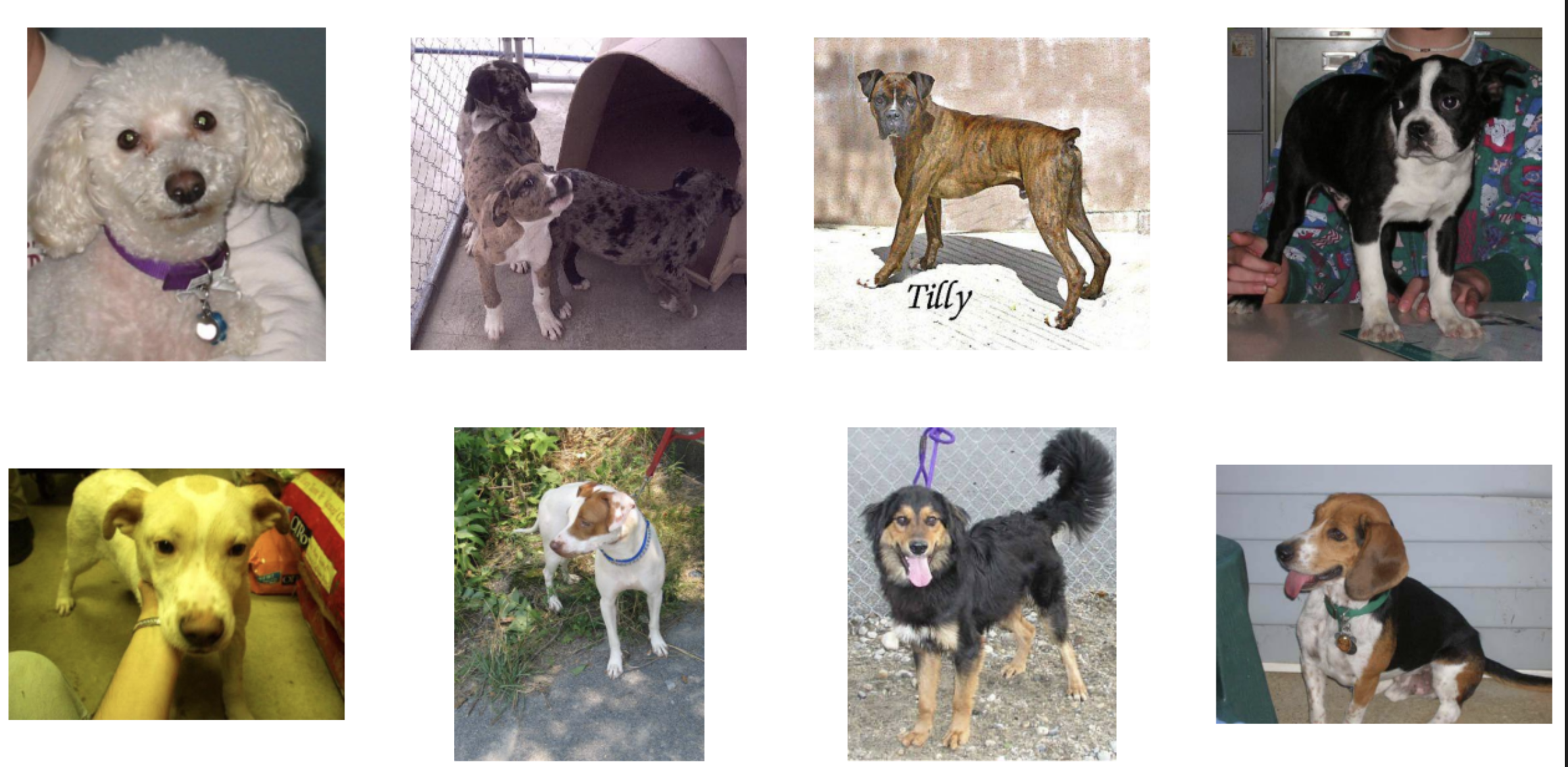
이제 고양이와 개 데이터세트가 어떻게 생겼는지 더 잘 이해하기 위해 몇 장의 사진을 살펴본다. 먼저 matplotlib 매개변수를 구성한다.

%matplotlib inline

import matplotlib.image as mpimg
import matplotlib.pyplot as plt

# Parameters for our graph; we'll output images in a 4x4 configuration
nrows = 4
ncols = 4

pic_index = 0 # Index for iterating over images

# Set up matplotlib fig, and size it to fit 4x4 pics
fig = plt.gcf()
fig.set_size_inches(ncols*4, nrows*4)

pic_index+=8

next_cat_pix = [os.path.join(train_cats_dir, fname) 
                for fname in train_cat_fnames[ pic_index-8:pic_index] 
               ]

next_dog_pix = [os.path.join(train_dogs_dir, fname) 
                for fname in train_dog_fnames[ pic_index-8:pic_index]
               ]

for i, img_path in enumerate(next_cat_pix+next_dog_pix):
  # Set up subplot; subplot indices start at 1
  sp = plt.subplot(nrows, ncols, i + 1)
  sp.axis('Off') # Don't show axes (or gridlines)

  img = mpimg.imread(img_path)
  plt.imshow(img)

plt.show()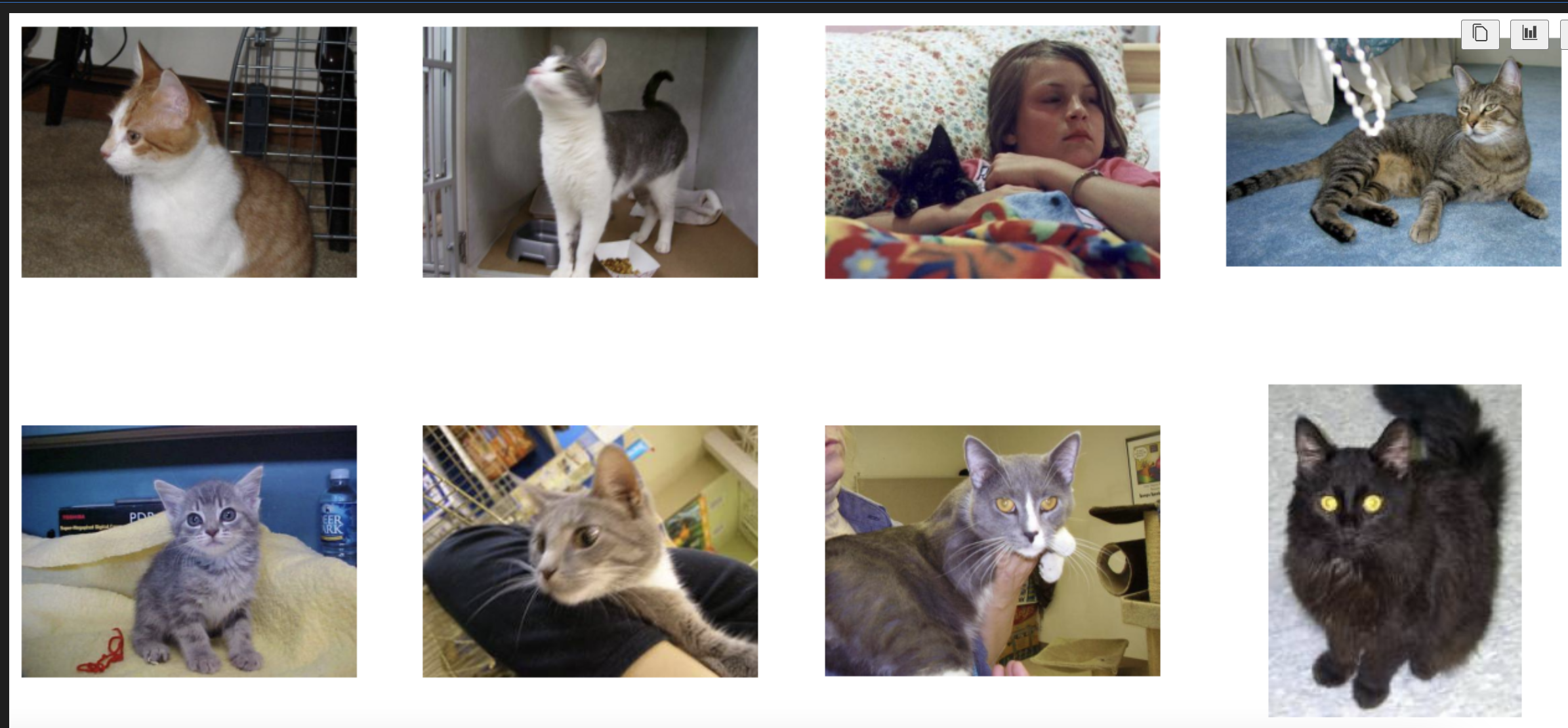

[2] 최대 72%의 정확도를 얻기 위해 처음부터 작은 모델 구축

이미지를 처리하도록 신경망을 훈련하려면 해당 이미지가 균일한 크기여야 한다. 이를 위해 150x150 픽셀을 선택하면 이미지를 해당 모양으로 전처리하는 코드 표시된다.

Tensorflow를 가져오고 Keras API를 사용하여 모델을 정의할 수 있다.

import tensorflow as  tf

model = tf.keras.models.Sequential([
    tf.keras.layers.Conv2D(16, (3,3), input_shape=(150,150,3), activation='relu'),
    tf.keras.layers.MaxPooling2D(2,2),
    tf.keras.layers.Conv2D(32, (3,3), activation='relu'),
    tf.keras.layers.MaxPooling2D(2,2),
    tf.keras.layers.Conv2D(64, (3,3), activation='relu'),
    tf.keras.layers.MaxPooling2D(2,2),
    tf.keras.layers.Flatten(),
    tf.keras.layers.Dense(512, activation='relu'),
    tf.keras.layers.Dense(1, activation='sigmoid')
    
])

model.summary()

이전과 같이 Sequential 레이어를 정의하고 일부 컨벌루션 레이어를 추가했다.
이번에는 input_shape 매개변수로 컬러 이미지가 있으므로 여기에 150x150 크기와 색상 깊이에 3을 입력했다.
그런 다음 두 개의 컨벌루션 레이어를 추가하고 최종 결과를 평면화하여 조밀하게 연결된 레이어에 공급한다.

2 클래스 분류 문제, 즉 이진 분류 문제에 직면했기 때문에 시그모이드 활성화로 신경망을 종료한다.
신경망의 출력은 0과 1 사이의 단일 스칼라가 되며, 현재 이미지가 클래스 1(클래스 0이 아님)일 확률을 인코딩한다.

model.summary() 메서드를 사용하여 네트워크 아키텍처를 검토할 수 있습니다.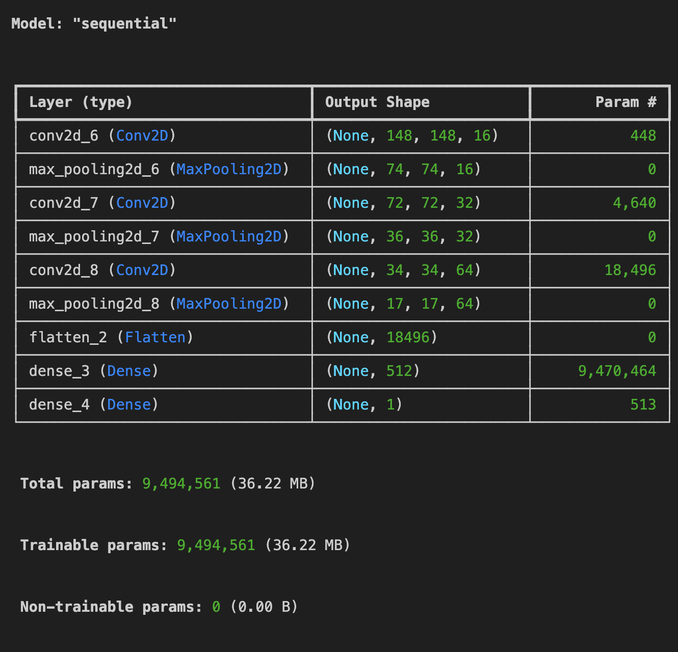

output_shape 열은 각 연속 레이어에서 feature map 의 크기가 어떻게 변화하는지 보여준다. 컨볼루션 작업은 원래 차원에서 가장 바깥쪽 픽셀을 제거하고 각 풀링 레이어는 이를 절반으로 줄인다.

다음으로 모델 학습을 위한 사양을 구성합니다. 이진 분류 문제이고 최종 활성화가 시그모이드이기 때문에 Binary_crossentropy 손실을 사용하여 모델을 학습한다. 학습률이 0.001인 rmsprop 옵티마이저를 사용한다.

model.compile(loss='binary_crossentropy',
              optimizer=tf.keras.optimizers.RMSprop(learning_rate=0.001),
              metrics=['accuracy'])

참고: 이 경우 RMSprop 최적화 알고리즘을 사용하는 것이 SGD(확률적 경사하강법)보다 더 좋다. RMSprop이 학습 속도 조정을 자동화하기 때문입니다. (Adam 및 Adagrad와 같은 다른 최적화 프로그램도 훈련 중에 학습 속도를 자동으로 조정하며 여기서도 똑같이 잘 작동한다.)

[3] data preprocessing

다음 단계는 소스 폴더의 그림을 읽고, 이를 float32 텐서로 변환하고, 해당 레이블과 함께 모델에 공급하는 데이터 생성기를 설정하는 것이다.
훈련 이미지용 생성기 하나와 검증 이미지용 생성기 하나가 있다. 이 생성기는 150x150 크기의 이미지 배치와 해당 레이블(바이너리)을 생성한다.

이미 알고 있듯이 신경망에 들어가는 데이터는 일반적으로 신경망 처리에 더 적합하도록 어떤 방식으로든 정규화되어야 한다(예: 원시 픽셀을 ConvNet에 공급하는 것은 일반적이지 않다). 픽셀 값을 [0, 1] 범위에 있도록 정규화하여 이미지를 생성한다(원래 모든 값은 [0, 255] 범위에 있음).

Keras에서는 rescale 매개변수를 사용하는 keras.preprocessing.image.ImageDataGenerator 클래스를 통해 이 작업을 수행할 수 있다. 이 ImageDataGenerator 클래스를 사용하면 .flow(data, labels) 또는 .flow_from_directory(directory)를 통해 증강 이미지 배치(및 해당 레이블)의 생성기를 인스턴스화할 수 있다.

from tensorflow.keras.preprocessing.image import ImageDataGenerator

train_datagen = ImageDataGenerator(rescale=1.0/255.)
test_datagen = ImageDataGenerator(rescale=1.0/255.)

train_generator = train_datagen.flow_from_directory(
    train_dir,
    target_size=(150,150),
    batch_size=20,
    class_mode= 'binary'
)

test_generator = train_datagen.flow_from_directory(
    validation_dir,
    target_size = (150,150),
    batch_size=20,
    class_mode='binary'
)

#output

Found 2000 images belonging to 2 classes.
Found 1000 images belonging to 2 classes.

[4] model Training

이제 15개 epcoh 동안 사용 가능한 2,000개의 이미지를 모두 학습하고 검증 세트의 1,000개 이미지에 대한 정확도도 모니터링한다.

손실, 정확도, 검증 손실, 검증 정확도 등 에포크당 4가지 값이 표시된다.

손실과 정확성은 훈련 진행 상황을 나타내는 훌륭한 지표이다. 손실은 알려진 레이블에 대한 현재 모델 예측을 측정하여 결과를 계산한다. 반면에 정확도는 정확한 추측의 일부이다.

history = model.fit(
    train_generator,
    epochs=15,
    validation_data = test_generator,
    verbose=2
)

[5] Model prediction

이제 모델을 사용하여 실제로 예측을 실행하는 방법이다. 이 코드를 사용하면 파일 시스템에서 하나 이상의 파일을 선택하고, 업로드하고, 모델을 통해 실행하여 개체가 고양이인지 개인지 표시할 수 있다.

import numpy as np
from tensorflow.keras.utils import load_img, img_to_array

cat_path = './cats_and_dogs_filtered/validation/cats/'
dog_path = './cats_and_dogs_filtered/validation/dogs/'

cat_fileName = os.listdir('./cats_and_dogs_filtered/validation/cats')[10]
dog_fileName = os.listdir('./cats_and_dogs_filtered/validation/dogs')[40]

path1 = cat_path + cat_fileName
path2 = dog_path + dog_fileName

for path in [path1,path2]:
    img = load_img(path, target_size=(150, 150))
    x = img_to_array(img)
    x /= 255
    x = np.expand_dims(x, axis=0)

    images = np.vstack([x])
    classes = model.predict(images, batch_size=10)

    print(classes[0])
    if classes[0] > 0.5:
        print("The image is a dog")
    else:
        print("The image is a cat")

validation data에 있는 고양이과 개 데이터를 랜덤으로 골라 해당 모델의 예측값을 살펴보았다.

img = mpimg.imread(path1)
plt.imshow(img)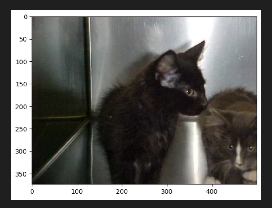 

img = mpimg.imread(path2)
plt.imshow(img)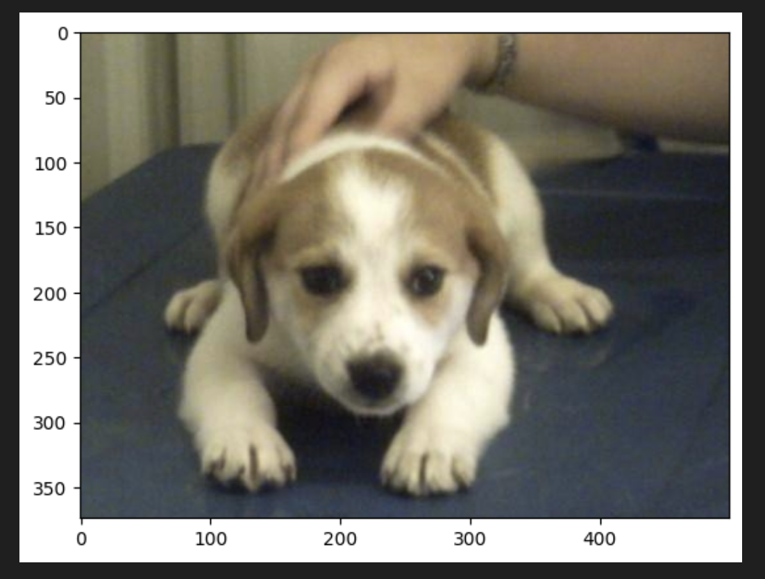

고양이과 개를 잘 분류하는 것을 볼 수 있다.

[6] Visualizaing Intermediate Representations**

import numpy as np
import random
from tensorflow.keras.utils import img_to_array, load_img

# Define a new Model that will take an image as input, and will output
# intermediate representations for all layers in the previous model
successive_outputs = [layer.output for layer in model.layers]
visualization_model = tf.keras.models.Model(inputs = model.inputs, outputs = successive_outputs)

# Prepare a random input image from the training set.
cat_img_files = [os.path.join(train_cats_dir, f) for f in train_cat_fnames]
dog_img_files = [os.path.join(train_dogs_dir, f) for f in train_dog_fnames]
img_path = random.choice(cat_img_files + dog_img_files)
img = load_img(img_path, target_size=(150, 150))  # this is a PIL image
x   = img_to_array(img)                           # Numpy array with shape (150, 150, 3)
x   = x.reshape((1,) + x.shape)                   # Numpy array with shape (1, 150, 150, 3)

# Scale by 1/255
x /= 255.0

# Run the image through the network, thus obtaining all
# intermediate representations for this image.
successive_feature_maps = visualization_model.predict(x)

# These are the names of the layers, so you can have them as part of our plot
layer_names = [layer.name for layer in model.layers]

# Display the representations
for layer_name, feature_map in zip(layer_names, successive_feature_maps):
  
  if len(feature_map.shape) == 4:
    
    #-------------------------------------------
    # Just do this for the conv / maxpool layers, not the fully-connected layers
    #-------------------------------------------
    n_features = feature_map.shape[-1]  # number of features in the feature map
    size       = feature_map.shape[ 1]  # feature map shape (1, size, size, n_features)
    
    # Tile the images in this matrix
    display_grid = np.zeros((size, size * n_features))
    
    #-------------------------------------------------
    # Postprocess the feature to be visually palatable
    #-------------------------------------------------
    for i in range(n_features):
      x  = feature_map[0, :, :, i]
      x -= x.mean()
      x /= x.std ()
      x *=  64
      x += 128
      x  = np.clip(x, 0, 255).astype('uint8')
      display_grid[:, i * size : (i + 1) * size] = x # Tile each filter into a horizontal grid

    #-----------------
    # Display the grid
    #-----------------
    scale = 20. / n_features
    plt.figure( figsize=(scale * n_features, scale) )
    plt.title ( layer_name )
    plt.grid  ( False )
    plt.imshow( display_grid, aspect='auto', cmap='viridis' )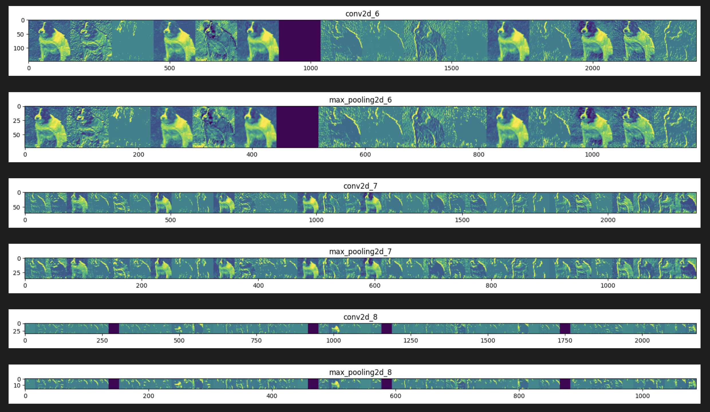 

• 위에서 강조 표시된 픽셀이 특히 하단 그리드에서 점점 더 추상적이고 컴팩트한 표현으로 바뀌는 것을 볼 수 있다.

• 다운스트림 표현은 신경망이 주의를 기울이는 부분을 강조하기 시작하고 "활성화"되는 기능의 수가 점점 더 적어진다. 대부분은 0으로 설정되어 있다. 이를 표현 희소성(representation sparsity)이라고 하며 딥러닝의 핵심 기능이다. 이러한 표현은 이미지의 원본 픽셀에 대한 정보를 점점 더 적게 전달하지만 이미지 클래스에 대한 정보는 점점 더 정교해진다. Conv2D(또는 일반적으로 심층 네트워크)을 각 계층이 가장 유용한 기능을 필터링하는 정보 증류 파이프라인으로 생각할 수 있다.

[7] Evaluating Accuracy and Loss for the Model

#-----------------------------------------------------------
# Retrieve a list of list results on training and test data
# sets for each training epoch
#-----------------------------------------------------------
acc      = history.history[     'accuracy' ]
val_acc  = history.history[ 'val_accuracy' ]
loss     = history.history[    'loss' ]
val_loss = history.history['val_loss' ]

epochs   = range(len(acc)) # Get number of epochs

#------------------------------------------------
# Plot training and validation accuracy per epoch
#------------------------------------------------
plt.plot  ( epochs,acc)
plt.plot  ( epochs, val_acc, color='red' )
plt.title ('Training and validation accuracy')
plt.figure()

#------------------------------------------------
# Plot training and validation loss per epoch
#------------------------------------------------
plt.plot  ( epochs,loss)
plt.plot  ( epochs, val_loss,color='red' )
plt.title ('Training and validation loss'   )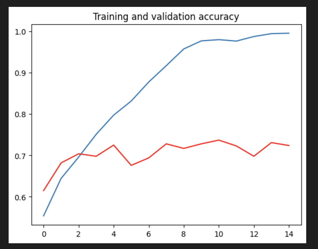

0.75 정도이고 에포크 2에서부터 유의미한 학습이 아니다.
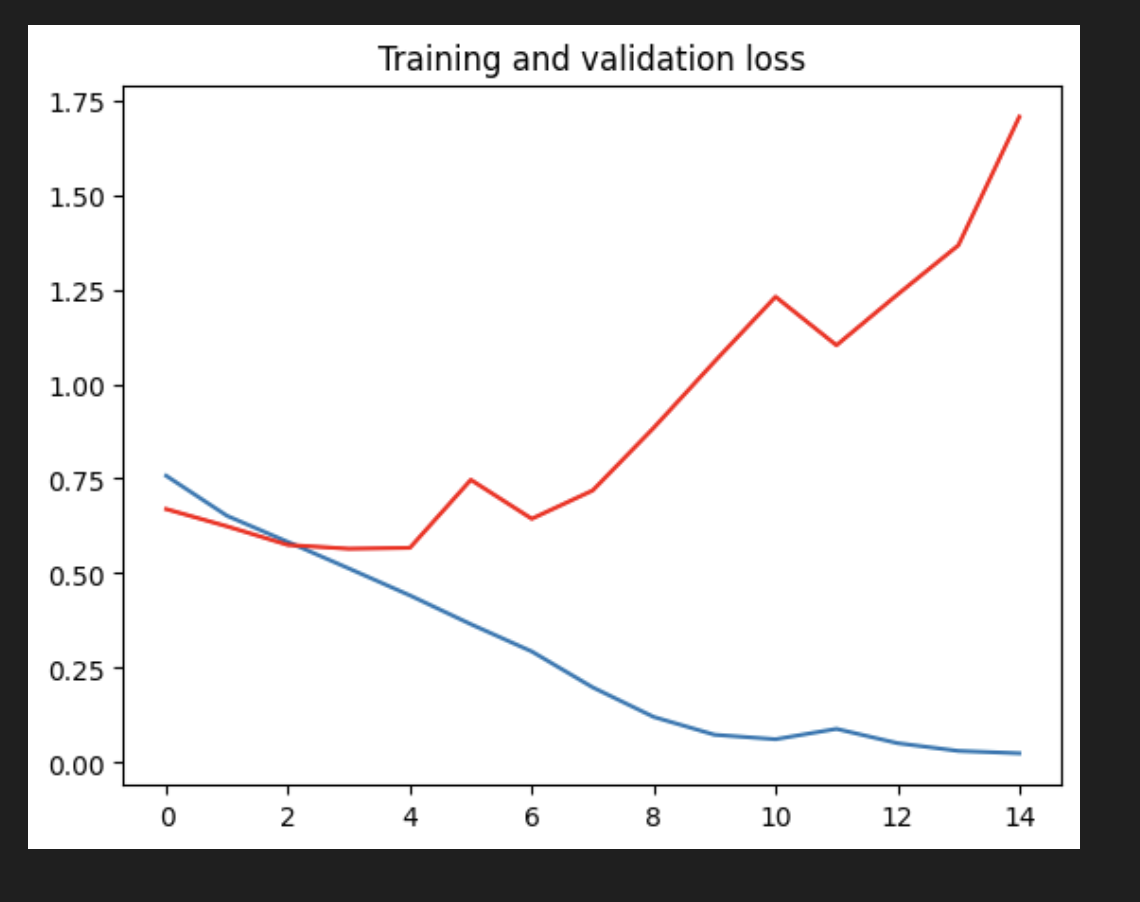
검증 손실값이 증가했고, 2번 epoch 이후 정확도가 75% 로부터 증가하지 않고 있으므로 유의미한 학습이 아니다.

• 그래프를 보면 모델이 과적합되어 있는 것을 볼 수 있다. 훈련 정확도(파란색)는 100%에 가까워지는 반면 검증 정확도(빨간색)는 70%에 머물고 있다. 검증 손실은 단 5번의 에포크 후에 최소값에 도달한다.

상대적으로 적은 수의 훈련 예제(2000)를 갖고 있으므로 과적합이 큰 문제이다. 과적합은 너무 적은 수의 예에 노출된 모델이 새로운 데이터에 일반화되지 않는 패턴을 학습할 때, 즉 모델이 예측을 위해 관련 없는 기능을 사용하기 시작할 때 발생한다.

과대적합은 기계 학습의 핵심 문제이다. 모델의 매개변수를 주어진 데이터 세트에 맞추는 경우, 모델에서 학습한 표현이 이전에 본 적이 없는 데이터에 적용 할 수 있을까? 훈련 데이터에 특정한 것을 학습하는 것을 어떻게 피할수 있을까?

다음 장에서는 이 분류 모델에서 과적합을 방지하는 방법을 살펴본다.