[Tensorflow] 4. Sequences, Time Series and Prediction (1 week Sequences and Prediction) : Programming (2)

[Tensorflow] 4. Sequences, Time Series and Prediction (1 week Sequences and Prediction) : Programming (2)

Statistical Forecasting on Synthetic Data(합성 데이터에 대한 통계적 예측)

• 여기서는 합성 시계열 데이터를 가지고 몇 가지 통계적 예측을 수행한다. 추후 머신러닝 기법과 비교하게 될 것이다.

[1] import & Utilities

필요한 라이브러리를 임포트하고 몇 가지 유틸리티 함수를 정의한다.

import tensorflow as tf
import numpy as np
import matplotlib.pyplot as plt

def plot_series(time, series, format="-", start=0, end=None):
    """
    Visualizes time series data

    Args:
      time (array of int) - contains the time steps
      series (array of int) - contains the measurements for each time step
      format - line style when plotting the graph
      label - tag for the line
      start - first time step to plot
      end - last time step to plot
    """

    # Setup dimensions of the graph figure
    plt.figure(figsize=(10, 6))
    
    if type(series) is tuple:

      for series_num in series:
        # Plot the time series data
        plt.plot(time[start:end], series_num[start:end], format)

    else:
      # Plot the time series data
      plt.plot(time[start:end], series[start:end], format)

    # Label the x-axis
    plt.xlabel("Time")

    # Label the y-axis
    plt.ylabel("Value")

    # Overlay a grid on the graph
    plt.grid(True)

    # Draw the graph on screen
    plt.show()

시계열 합성 데이터를 생성하기 위해 추세, 계절성, 노이즈를 추가하는 함수를 작성한다.

def trend(time, slope=0):
    """
    Generates synthetic data that follows a straight line given a slope value.

    Args:
      time (array of int) - contains the time steps
      slope (float) - determines the direction and steepness of the line

    Returns:
      series (array of float) - measurements that follow a straight line
    """

    # Compute the linear series given the slope
    series = slope * time

    return series

def seasonal_pattern(season_time):
    """
    Just an arbitrary pattern, you can change it if you wish
    
    Args:
      season_time (array of float) - contains the measurements per time step

    Returns:
      data_pattern (array of float) -  contains revised measurement values according 
                                  to the defined pattern
    """

    # Generate the values using an arbitrary pattern
    data_pattern = np.where(season_time < 0.4,
                    np.cos(season_time * 2 * np.pi),
                    1 / np.exp(3 * season_time))
    
    return data_pattern

def seasonality(time, period, amplitude=1, phase=0):
    """
    Repeats the same pattern at each period

    Args:
      time (array of int) - contains the time steps
      period (int) - number of time steps before the pattern repeats
      amplitude (int) - peak measured value in a period
      phase (int) - number of time steps to shift the measured values

    Returns:
      data_pattern (array of float) - seasonal data scaled by the defined amplitude
    """
    
    # Define the measured values per period
    season_time = ((time + phase) % period) / period

    # Generates the seasonal data scaled by the defined amplitude
    data_pattern = amplitude * seasonal_pattern(season_time)

    return data_pattern

def noise(time, noise_level=1, seed=None):
    """Generates a normally distributed noisy signal

    Args:
      time (array of int) - contains the time steps
      noise_level (float) - scaling factor for the generated signal
      seed (int) - number generator seed for repeatability

    Returns:
      noise (array of float) - the noisy signal
    """

    # Initialize the random number generator
    rnd = np.random.RandomState(seed)

    # Generate a random number for each time step and scale by the noise level
    noise = rnd.randn(len(time)) * noise_level
    
    return noise

[2] Generate the synthetic data(합성 데이터 생성)

• 위의 유틸리티 함수를 사용하여 합성 데이터를 생성한다. 기준선에서 시작한 다음 365단계마다 계절 패턴으로 상향 추세를 보이는 데이터이다. 실제 데이터에도 노이즈가 있는 경우가 많기 때문에 약간의 노이즈도 추가한다.

# Parameters
time = np.arange(4 * 365 + 1, dtype="float32")
baseline = 10
amplitude = 40
slope = 0.05
noise_level = 5

# Create the series
series = baseline + trend(time, slope) + seasonality(time, period=365, amplitude=amplitude)

# Update with noise
series += noise(time, noise_level, seed=42)

# Plot the results
plot_series(time, series)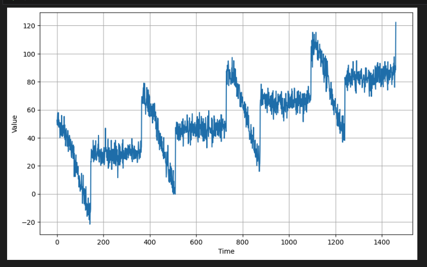

[3] Split the data

-위의 데이터를 훈련 및 검증 세트로 분할한다.
처음부터 1,000개의 데이터는 훈련용으로 사용하고 나머지는 검증용으로 사용한다.

split_time = 1000

time_train = time[:split_time]
x_train = series[:split_time]

time_valid = time[split_time:]
x_valid = series[split_time:]

플로팅에 동일한 유틸리티 기능을 사용하여 이러한 세트를 시각적으로 확인해본다.
일반적으로 검증 세트는 훈련 세트보다 더 높은 값(예: y축)을 갖는다. 모델은 훈련 세트의 추세와 계절성을 학습함으로써 이러한 값을 예측할 수 있어야 한다.

# Plot the train set
plot_series(time_train, x_train)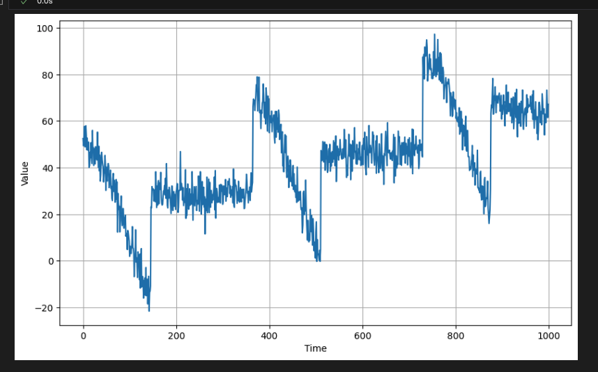

# Plot the validation set
plot_series(time_valid, x_valid)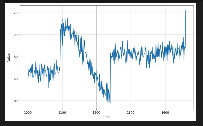

검증 데이터의 y축의 수치가 학습 데이터보다 높은 것을 볼 수 있다.

[4] Navie Forcast

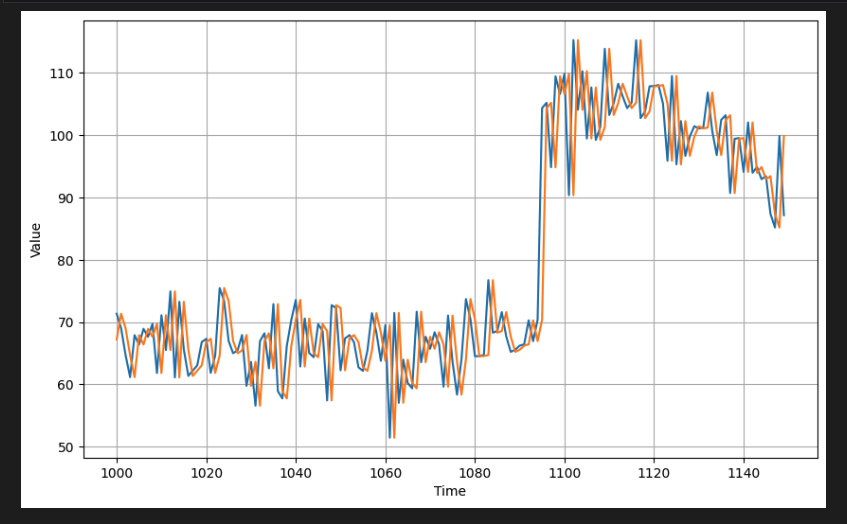
• 기준선으로 다음 값이 이전 시간 단계와 동일할 것이라고 가정하는 navie한 예측을 수행할 수 있다.
  아래와 같이 원래 시간을 분할하고 일부 값을 인쇄할 수 있는데, 다음 시간 단계 값은 이전 시간 단계의 실제값과 동일해야 한다.

naive_forecast = series[split_time-1:-1]

time_step = 100

print(f"ground truth at time step {time_step} : {x_valid[time_step]}")
print(f"prediction at time step {time_step+1} : {naive_forecast[time_step+1]}")

# output
ground truth at time step 100 : 109.84197998046875
prediction at time step 101 : 109.84197998046875

앞서 정의한 plot_series() 함수를 사용하면 이를 시각적으로 확인해보자.

plot_series(time_valid, (x_valid, naive_forecast))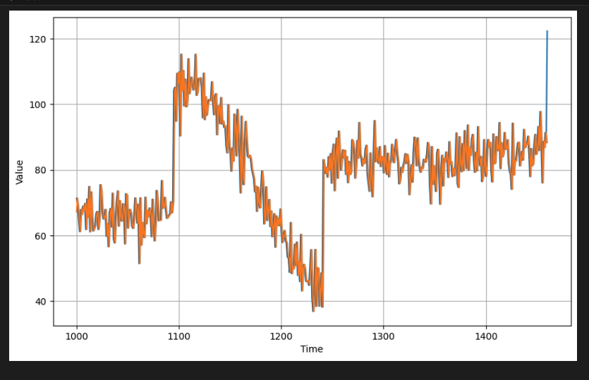

plot_series(time_valid, (x_valid, naive_forecast))

검증 기간이 시작될 때 확대하여 naive한 예측이 시계열보다 1단계 뒤처지는 것을 확인할 수 있다.

[5] computing metrics

• 이제 검증 기간의 예측과 예측 간의 측정 지표는
  '평균 제곱 오차(MSE)'와 '평균 절대 오차('MAE)'를 계산한다. 이는 tf.keras.metrics API를 통해 사용할 수 있다.

print(tf.keras.metrics.mean_squared_error(x_valid, naive_forecast).numpy())
print(tf.keras.metrics.mean_absolute_error(x_valid, naive_forecast).numpy())

# output
61.827534
5.9379086

• 위의 값은 기준이 되며 다른 방법을 사용하여 navie한 예측보다 더 나은 결과를 얻을 수 있는지 확인할 수 있다.

[6] Moving Average(이동 평균)

• 사용할 수 있는 한 가지 기술은 이동 평균이다.
  이동 평균은 일련의 시간 단계를 요약하는 것이다. 평균은 다음 시간 단계에 대한 예측이 된다.
  예를 들어, 시간 단계 1~10의 측정값 평균은 시간 단계 11에 대한 예측이 되고, 시간 단계 2~11에 대한 평균은 시간 단계 12에 대한 예측이 된다.

• 아래 함수는 전체 계열에 대한 이동 평균을 수행하는 것이다. 평균을 계산할 때 고려해야 할 시간 단계 수를 나타내려면 window_size 인수가 필요하다.

def moving_average_forecast(series, window_size):
    """Generates a moving average forecast

    Args:
      series (array of float) - contains the values of the time series
      window_size (int) - the number of time steps to compute the average for

    Returns:
      forecast (array of float) - the moving average forecast
    """

    # Initialize a list
    forecast = []
    
    # Compute the moving average based on the window size
    for time in range(len(series) - window_size):
      forecast.append(series[time:time + window_size].mean())
    
    # Convert to a numpy array
    forecast = np.array(forecast)

    return forecast

이 함수를 사용하여 창 크기가 30인 예측을 생성해보자.

# Generate the moving average forecast
moving_avg = moving_average_forecast(series, 30)[split_time - 30:]

# Plot the results
plot_series(time_valid, (x_valid, moving_avg))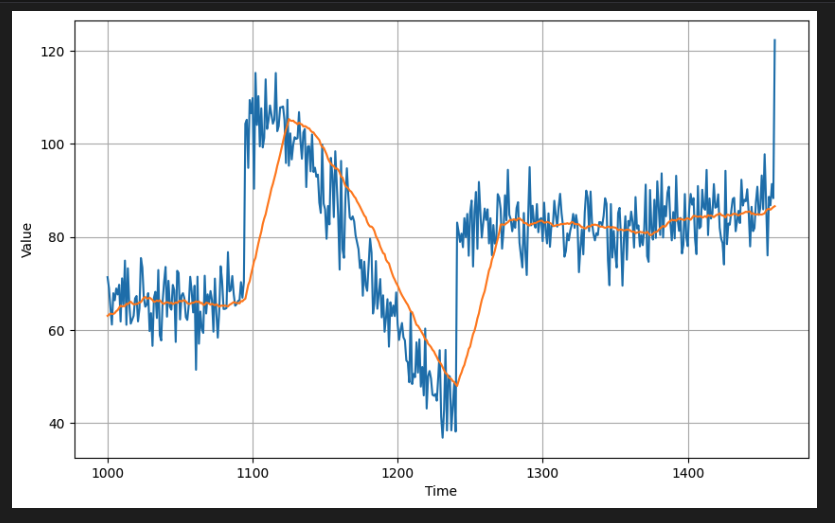

# Compute the metrics
print(tf.keras.metrics.mean_squared_error(x_valid, moving_avg).numpy())
print(tf.keras.metrics.mean_absolute_error(x_valid, moving_avg).numpy())

# output
106.674576
7.1424184

여기서는 navie한 예측보다 더 나쁜 수치를 보여주는 것을 볼 수 있다. 이동 평균은 추세나 계절성을 예측하지 않는다.
특히, 원본 데이터의 이러한 큰 급증은 위의 플롯에서 볼 수 있듯이 큰 편차를 유발한다. 시간 차이를 통해 데이터 세트의 이러한 특성을 제거하고 더 나은 결과를 얻을 수 있는지 확인해보자.

[7] Differencing(차분)

• 계절성 기간이 365일이므로 시간 t의 값에서 시간 t – 365의 값을 뺀다.
  또한 결과를 시간 배열에 맞춰 정렬해야 한다. t >= 365에 대해서만 시간 차이를 수행할 수 있으므로 시간 배열의 처음 365개 시간 단계를 잘라야 한다.

diff_series = (series[365:] - series[:-365])

diff_time = time[365:]

plot_series(diff_time, diff_series)

• 결과를 플롯하여 값을 시각화 해본다.
  

• 추세와 계절성이 사라진 것을 볼 수 있다. 이제 이동 평균을 사용하여 다시 시도 해본다. diff_series는 실제값이고 diff_moving_avg는 예측 배열이다. 비교하기 전에 검증 세트 시간 단계에 해당하도록 이를 적절하게 분할한다.

# Generate moving average from the time differenced dataset
diff_moving_avg = moving_average_forecast(diff_series, 30)

# Slice the prediction points that corresponds to the validation set time steps
diff_moving_avg = diff_moving_avg[split_time - 365 - 30:]

# Slice the ground truth points that corresponds to the validation set time steps
diff_series = diff_series[split_time - 365:]

# Plot the results
plot_series(time_valid, (diff_series, diff_moving_avg))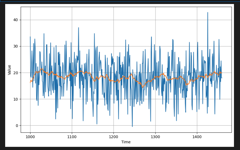

이제 t – 365의 과거 값을 추가하여 추세와 계절성을 다시 가져온다.