[Tensorflow] 4. Sequences, Time Series and Prediction (1 week Sequences and Prediction) : Programming (1)

[Tensorflow] 4. Sequences, Time Series and Prediction (1 week Sequences and Prediction) : Programming (1)

Introduction to Time Series Plots(시계열 도표 소개)

• 여기서는 합성 데이터를 생성해서, 시계열의 다양한 용어와 속성을 알아본다.

[1] import & Plot Utilities

import numpy as np
import matplotlib.pyplot as plt

def plot_series(time, series, format="-", start=0, end=None, label=None):
    """
    Visualizes time series data

    Args:
      time (array of int) - contains the time steps
      series (array of int) - contains the measurements for each time step
      format (string) - line style when plotting the graph
      start (int) - first time step to plot
      end (int) - last time step to plot
      label (list of strings)- tag for the line
    """

    # Setup dimensions of the graph figure
    plt.figure(figsize=(10, 6))

    # Plot the time series data
    plt.plot(time[start:end], series[start:end], format)

    # Label the x-axis
    plt.xlabel("Time")

    # Label the y-axis
    plt.ylabel("Value")

    if label:
      plt.legend(fontsize=14, labels=label)

    # Overlay a grid on the graph
    plt.grid(True)

    # Draw the graph on screen
    plt.show()

[2] Trend (추세)

• 추세는 시간이 지남에 따라 값이 올라가거나 내려가는 일반적인 경향이다.
  특정 기간이 주어지면 그래프가 상승/양수 추세, 하락/음수 추세 또는 평면을 따르는지 확인할 수 있다.
  예를 들어, 좋은 위치에 있는 주택 가격은 시간이 지남에 따라 전반적인 가치 상승을 볼 수 있다.

• 시각화할 수 있는 가장 간단한 예는 직선을 따르는 데이터이다.
  이를 생성하기 위해 아래 함수를 사용하는데, 기울기 인수는 추세가 무엇인지 결정한다. 해당 함수를 y 절편이 0인 기울기 절편 형식으로 인식할 수 있다.

def trend(time, slope=0):
    """
    Generates synthetic data that follows a straight line given a slope value.

    Args:
      time (array of int) - contains the time steps
      slope (float) - determines the direction and steepness of the line

    Returns:
      series (array of float) - measurements that follow a straight line
    """

    # Compute the linear series given the slope
    series = slope * time

    return series

상승 추세를 보이는 시계열을 그려보자.
하향 추세의 경우 아래 기울기 값을 음수 값(예: -0.3)으로 바꾸면 된다.

# Generate time steps. Assume 1 per day for one year (365 days)
time = np.arange(365)

# Define the slope (You can revise this)
slope = 0.1

# Generate measurements with the defined slope
series = trend(time, slope)

# Plot the results
plot_series(time, series, label=[f'slope={slope}'])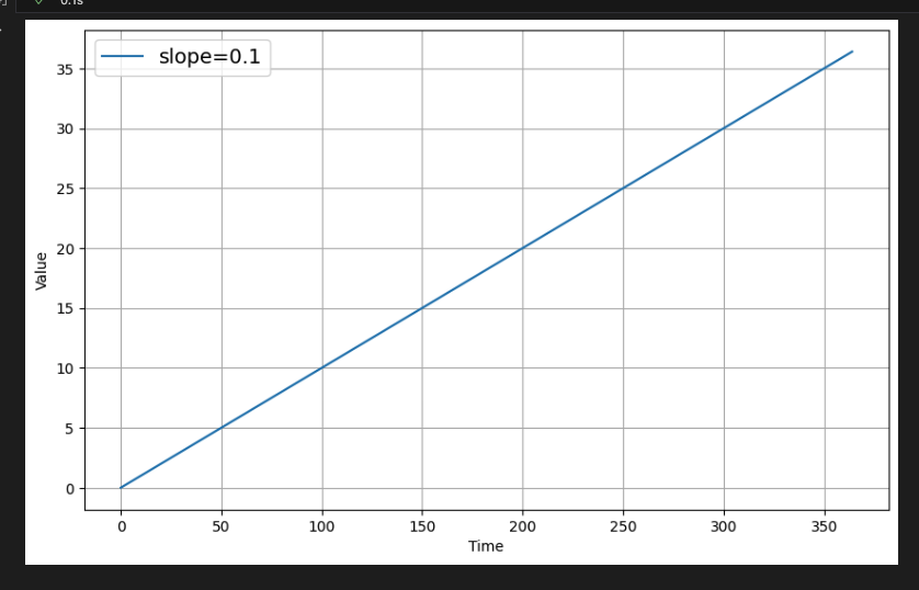

# Generate time steps. Assume 1 per day for one year (365 days)
time = np.arange(365)
slope = -0.3
series = trend(time, slope)
plot_series(time, series, label=[f'slope={slope}'])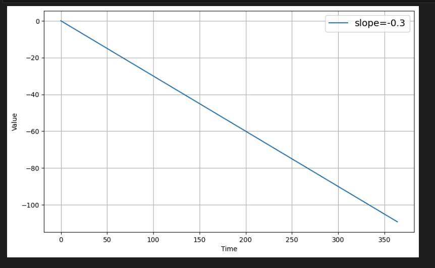

이 동작을 모델링하는 데는 기계 학습이 필요하지 않고, 간단히 선의 방정식을 풀면 완벽한 예측 모델을 얻을 수 있다. 이와 같은 데이터는 실제 응용 프로그램에서는 극히 드물며 추세선은 수업 중 무어의 법칙 예제에 표시된 것과 같은 지침으로만 사용된다.

[3] Seasonality (계절성)

• 계절성은 일정한 시간 간격으로 반복되는 패턴이다.
  예를 들어, 시간당 온도는 연속 10일 동안 비슷하게 변동할 수 있으며 이를 사용하여 다음 날의 행동을 예측할 수 있다.
  아래 함수를 사용하여 계절 패턴이 있는 시계열을 생성할 수 있다.

def seasonal_pattern(season_time):
    """
    Just an arbitrary pattern, you can change it if you wish
    
    Args:
      season_time (array of float) - contains the measurements per time step

    Returns:
      data_pattern (array of float) -  contains revised measurement values according 
                                  to the defined pattern
    """

    # Generate the values using an arbitrary pattern
    data_pattern = np.where(season_time < 0.4,
                    np.cos(season_time * 2 * np.pi),
                    1 / np.exp(3 * season_time))
    
    return data_pattern

def seasonality(time, period, amplitude=1, phase=0):
    """
    Repeats the same pattern at each period

    Args:
      time (array of int) - contains the time steps
      period (int) - number of time steps before the pattern repeats
      amplitude (int) - peak measured value in a period
      phase (int) - number of time steps to shift the measured values

    Returns:
      data_pattern (array of float) - seasonal data scaled by the defined amplitude
    """
    
    # Define the measured values per period
    season_time = ((time + phase) % period) / period

    # Generates the seasonal data scaled by the defined amplitude
    data_pattern = amplitude * seasonal_pattern(season_time)

    return data_pattern

365개 시간 단계마다 패턴을 볼 수 있으므로 생성된 데이터의 계절성을 보여준다.

• 시계열에는 추세와 계절성이 모두 포함될 수도 있다.
  예를 들어, 시간당 기온은 짧은 기간 동안 규칙적으로 변동할 수 있지만 다년간의 데이터를 보면 상승 추세를 보일 수 있다.

아래 예는 상승 추세가 있는 계절적 패턴을 보여줍니다.

# Define seasonal parameters
slope = 0.05
period = 365
amplitude = 40

# Generate the data
series = trend(time, slope) + seasonality(time, period=period, amplitude=amplitude)

# Plot the results
plot_series(time, series)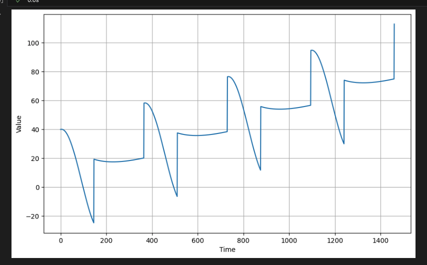

[4] Noise (노이즈)

• 실제로 매끄러운 신호를 갖는 실제 시계열은 거의 없다.
  일반적으로 해당 신호에 약간의 잡음인 노이즈가 있는데, 잡음(노이즈)가 있는 신호는 아래와 같다.

def noise(time, noise_level=1, seed=None):
    """Generates a normally distributed noisy signal

    Args:
      time (array of int) - contains the time steps
      noise_level (float) - scaling factor for the generated signal
      seed (int) - number generator seed for repeatability

    Returns:
      noise (array of float) - the noisy signal

    """

    # Initialize the random number generator
    rnd = np.random.RandomState(seed)

    # Generate a random number for each time step and scale by the noise level
    noise = rnd.randn(len(time)) * noise_level
    
    return noise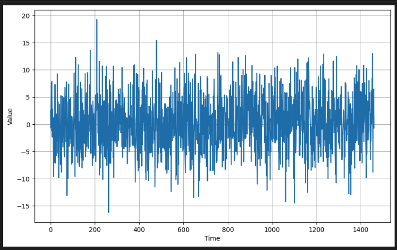

이전에 생성한 시계열에 노이즈를 추가해본다.

# Add the noise to the time series
series += noise_signal

# Plot the results
plot_series(time, series)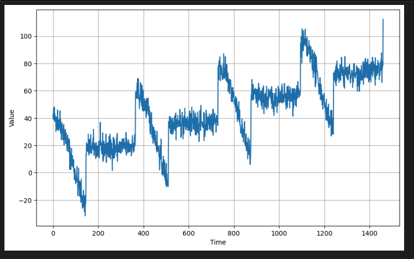

[5] Autocorrlation(자기 상관성)

• 시계열은 자기상관성을 가질 수 있다. 자기 상관성은 주어진 시간 단계에서의 측정값이 이전 시간 단계의 함수라는 것이다.
  이전 시간 단계의 계산이 발생하는 곳이기 때문에 단계 변수를 참조하는 행을 보면 되는데, 결과를 좀 더 현실적으로 만들기 위해 노이즈(예: 난수)를 포함한 코드이다.

def autocorrelation(time, amplitude, seed=None):
    """
    Generates autocorrelated data

    Args:
      time (array of int) - contains the time steps
      amplitude (float) - scaling factor
      seed (int) - number generator seed for repeatability

    Returns:
      ar (array of float) - autocorrelated data
    """

    # Initialize random number generator 
    rnd = np.random.RandomState(seed)
    
    # Initialize array of random numbers equal to the length 
    # of the given time steps plus 50
    ar = rnd.randn(len(time) + 50)
    
    # Set first 50 elements to a constant
    ar[:50] = 100
    
    # Define scaling factors
    phi1 = 0.5
    phi2 = -0.1

    # Autocorrelate element 51 onwards with the measurement at 
    # (t-50) and (t-30), where t is the current time step
    for step in range(50, len(time) + 50):
        ar[step] += phi1 * ar[step - 50]
        ar[step] += phi2 * ar[step - 33]
    
    # Get the autocorrelated data and scale with the given amplitude.
    # The first 50 elements of the original array is truncated because
    # those are just constant and not autocorrelated.
    ar = ar[50:] * amplitude

    return ar

# Use time steps from previous section and generate autocorrelated data
series = autocorrelation(time, amplitude=10, seed=42)

# Plot the first 200 elements to see the pattern more clearly
plot_series(time[:200], series[:200])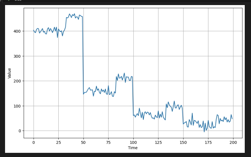

아래는 이전 시간 단계에서 값을 계산하는 보다 간단한 자기상관 함수이다.

def autocorrelation(time, amplitude, seed=None):
    """
    Generates autocorrelated data

    Args:
      time (array of int) - contains the time steps
      amplitude (float) - scaling factor
      seed (int) - number generator seed for repeatability

    Returns:
      ar (array of float) - generated autocorrelated data
    """

    # Initialize random number generator 
    rnd = np.random.RandomState(seed)

    # Initialize array of random numbers equal to the length 
    # of the given time steps plus an additional step
    ar = rnd.randn(len(time) + 1)

    # Define scaling factor
    phi = 0.8

    # Autocorrelate element 11 onwards with the measurement at 
    # (t-1), where t is the current time step
    for step in range(1, len(time) + 1):
        ar[step] += phi * ar[step - 1]
    
    # Get the autocorrelated data and scale with the given amplitude.
    ar = ar[1:] * amplitude
    
    return ar

# Use time steps from previous section and generate autocorrelated data
series = autocorrelation(time, amplitude=10, seed=42)

# Plot the results
plot_series(time[:200], series[:200])

발생할 수 있는 또 다른 자기상관 시계열은 무작위 급증 이후 예측 가능하게 감소하는 시계열이다. 먼저 아래에서 이러한 스파이크를 생성하는 함수를 정의한다.

def impulses(time, num_impulses, amplitude=1, seed=None):
    """
    Generates random impulses

    Args:
      time (array of int) - contains the time steps
      num_impulses (int) - number of impulses to generate
      amplitude (float) - scaling factor
      seed (int) - number generator seed for repeatability

    Returns:
      series (array of float) - array containing the impulses
    """

    # Initialize random number generator 
    rnd = np.random.RandomState(seed)

    # Generate random numbers
    impulse_indices = rnd.randint(len(time), size=num_impulses)

    # Initialize series
    series = np.zeros(len(time))

    # Insert random impulses
    for index in impulse_indices:
        series[index] += rnd.rand() * amplitude

    return series    

위의 함수를 사용하여 10개의 무작위 임펄스가 포함된 값을 생성한다.

# Generate random impulses
impulses_signal = impulses(time, num_impulses=10, seed=42)

# Plot the results
plot_series(time, impulses_signal)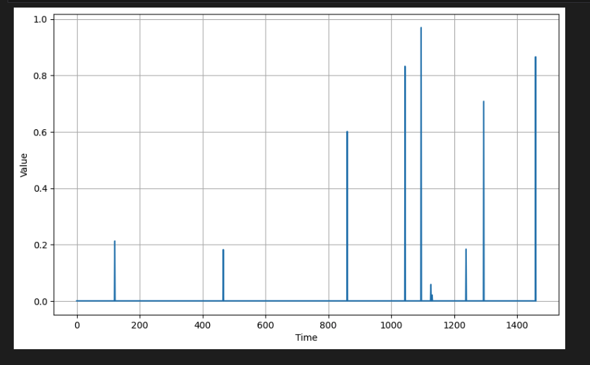

def autocorrelation_impulses(source, phis):
    """
    Generates autocorrelated data from impulses

    Args:
      source (array of float) - contains the time steps with impulses
      phis (dict) - dictionary containing the lag time and decay rates

    Returns:
      ar (array of float) - generated autocorrelated data
    """

    # Copy the source
    ar = source.copy()

    # Compute new series values based on the lag times and decay rates
    for step, value in enumerate(source):
        for lag, phi in phis.items():
            if step - lag > 0:
              ar[step] += phi * ar[step - lag]

    return ar

그런 다음 이 함수를 사용하여 스파이크 이후의 붕괴를 생성할 수 있다. 다음은 이전 시간 단계(예: t-1, 여기서 t는 현재 시간 단계)에서 다음 값을 생성하는 예시이다.

# Use the impulses from the previous section and generate autocorrelated data
series = autocorrelation_impulses(impulses_signal, {1: 0.99})

# Plot the results
plot_series(time, series)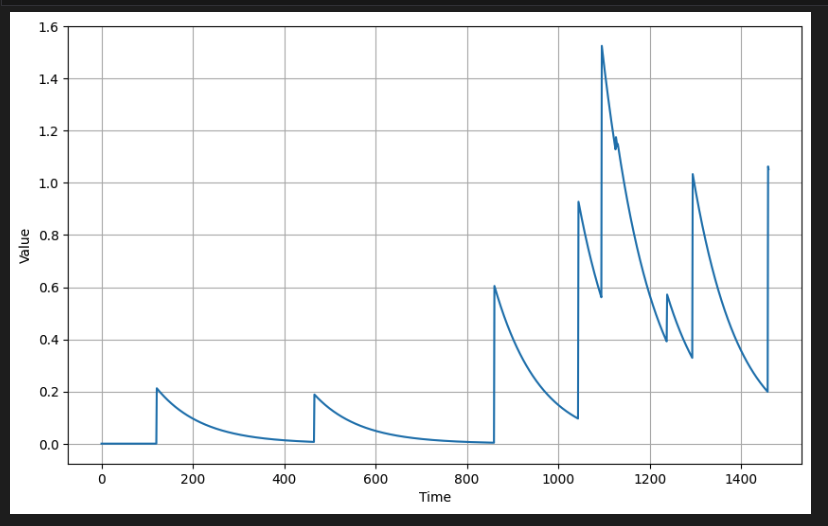

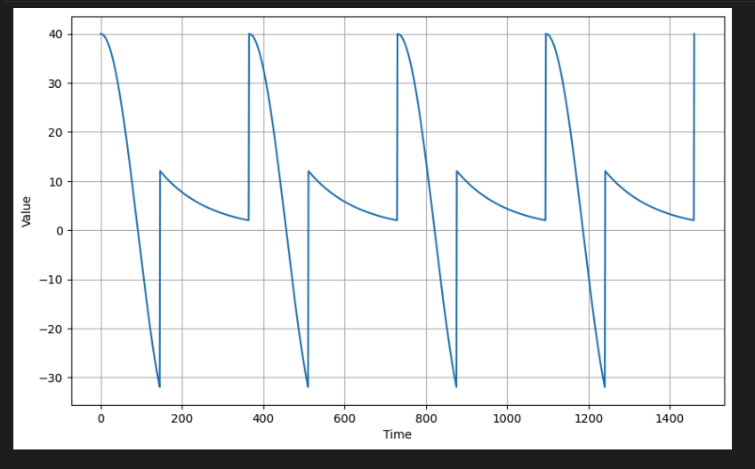
다음은 t-1 및 t-50의 값에서 다음 값을 계산하는 또 다른 예이다.

# Use the impulses from the previous section and generate autocorrelated data
series = autocorrelation_impulses(impulses_signal, {1: 0.70, 50: 0.2})

# Plot the results
plot_series(time, series)

자기 상관 데이터도 추세선을 탈 수 있다.
아래는 추세선을 탄 자기 상관 데이터이다.

# Generate autocorrelated data with an upward trend
series = autocorrelation(time, 10, seed=42) + trend(time, 2)

# Plot the results
plot_series(time[:200], series[:200])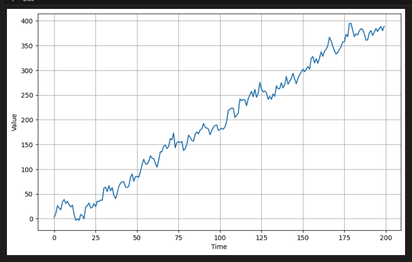

마찬가지로 이 데이터에 계절성을 추가할 수도 있다.

# Generate autocorrelated data with an upward trend
series = autocorrelation(time, 10, seed=42) + seasonality(time, period=50, amplitude=150) + trend(time, 2)

# Plot the results
plot_series(time[:200], series[:200])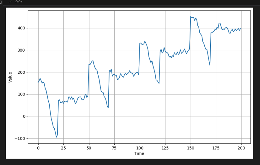

[6] Non-stationary Time Series(비정상 시계열)

• 시계열이 예상 패턴을 깨는 경우도 있는데, 대규모 이벤트는 데이터의 추세나 계절적 동작을 변경할 수 있다. 아래는 timstep = 200에서 그래프가 하향 추세로 이동하는 경우이다.

# Generate data with positive trend
series = autocorrelation(time, 10, seed=42) + seasonality(time, period=50, amplitude=150) + trend(time, 2)

# Generate data with negative trend
series2 = autocorrelation(time, 5, seed=42) + seasonality(time, period=50, amplitude=2) + trend(time, -1) + 550

# Splice the downward trending data into the first one at time step = 200
series[200:] = series2[200:]

# Plot the result
plot_series(time[:300], series[:300])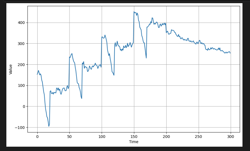

이와 같은 경우, 이후 단계(즉, t=200에서 시작)에서 모델을 학습할 수 있다. 미래 시간 단계에 대한 더 강력한 예측 신호를 제공하기 때문이다.