[Tensorflow] 4. Sequences, Time Series and Prediction(2. Deep Neural Networks for Time Series) : programminig (2)
Tensorflow_certification(텐서플로우 자격증)
[Tensorflow] 4. Sequences, Time Series and Prediction(2. Deep Neural Networks for Time Series) : programminig (2)
Training a Single Layer Neural Network with Time Series Data(시계열 데이터를 사용하여 단일 계층 신경망 훈련)
- 단일 신경망을 사용하여 시계열 데이터에 대한 예측 모델을 구축하는 방법을 사용한다.
단일 레이어 네트워크를 구축하고 합성 데이터를 사용하여 학습 시키기 위해 훈련 및 평가를 위한 시계열 데이터 준비를 진행하고 검증 세트를 기준으로 모델 성능을 측정한다.
[1] import & Utilities
시간에 대한 값을 플로팅할 수 있는 함수와 추세, 계절성, 노이즈를 만드는 유틸리티 함수를 정의한다.
이 함수를 통해서 시계열 데이터 및 모델 예측을 시각화하고 합성 데이터를 생성 한다.
def plot_series(time, series, format="-", start=0, end=None):
    """
    Visualizes time series data

    Args:
      time (array of int) - contains the time steps
      series (array of int) - contains the measurements for each time step
      format - line style when plotting the graph
      label - tag for the line
      start - first time step to plot
      end - last time step to plot
    """

    # Setup dimensions of the graph figure
    plt.figure(figsize=(10, 6))

    if type(series) is tuple:

      for series_num in series:
        # Plot the time series data
        plt.plot(time[start:end], series_num[start:end], format)

    else:
      # Plot the time series data
      plt.plot(time[start:end], series[start:end], format)

    # Label the x-axis
    plt.xlabel("Time")

    # Label the y-axis
    plt.ylabel("Value")

    # Overlay a grid on the graph
    plt.grid(True)

    # Draw the graph on screen
    plt.show()


def trend(time, slope=0):
    """
    Generates synthetic data that follows a straight line given a slope value.

    Args:
      time (array of int) - contains the time steps
      slope (float) - determines the direction and steepness of the line

    Returns:
      series (array of float) - measurements that follow a straight line
    """

    # Compute the linear series given the slope
    series = slope * time

    return series


def seasonal_pattern(season_time):
    """
    Just an arbitrary pattern, you can change it if you wish

    Args:
      season_time (array of float) - contains the measurements per time step

    Returns:
      data_pattern (array of float) -  contains revised measurement values according
                                  to the defined pattern
    """

    # Generate the values using an arbitrary pattern
    data_pattern = np.where(season_time < 0.4,
                    np.cos(season_time * 2 * np.pi),
                    1 / np.exp(3 * season_time))

    return data_pattern


def seasonality(time, period, amplitude=1, phase=0):
    """
    Repeats the same pattern at each period

    Args:
      time (array of int) - contains the time steps
      period (int) - number of time steps before the pattern repeats
      amplitude (int) - peak measured value in a period
      phase (int) - number of time steps to shift the measured values

    Returns:
      data_pattern (array of float) - seasonal data scaled by the defined amplitude
    """

    # Define the measured values per period
    season_time = ((time + phase) % period) / period

    # Generates the seasonal data scaled by the defined amplitude
    data_pattern = amplitude * seasonal_pattern(season_time)

    return data_pattern


def noise(time, noise_level=1, seed=None):
    """Generates a normally distributed noisy signal

    Args:
      time (array of int) - contains the time steps
      noise_level (float) - scaling factor for the generated signal
      seed (int) - number generator seed for repeatability

    Returns:
      noise (array of float) - the noisy signal
    """

    # Initialize the random number generator
    rnd = np.random.RandomState(seed)

    # Generate a random number for each time step and scale by the noise level
    noise = rnd.randn(len(time)) * noise_level

    return noise
[2] Generate the Synthetic Data
시계열 합성 데이터를 생성한다. 여기에는 추세, 계절성, 노이즈가 포함된 1,461개의 데이터 포인트가 포함된다.
# Parameters
time = np.arange(4 * 365 + 1, dtype="float32")
baseline = 10
amplitude = 40
slope = 0.05
noise_level = 5

# Create the series
series = baseline + trend(time, slope) + seasonality(time, period=365, amplitude=amplitude)

# Update with noise
series += noise(time, noise_level, seed=42)

# Plot the results
plot_series(time, series)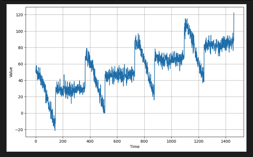
[3] Split the Dataset
- 위의 데이터를 훈련 및 검증 세트로 분할한다.
처음 1,000 포인트는 훈련용으로 사용하고 나머지는 검증용으로 사용한다.
split_time =1000

time_train= time[:split_time]
x_train = series[:split_time]

time_valid = time[split_time:]
x_valid = series[split_time:]

print(x_train.shape)
print(x_valid.shape)

# output
(1000,)
(461,)- 플로팅에 동일한 유틸리티 기능을 사용하여 이러한 세트를 시각적으로 확인할 수 있다. 일반적으로 검증 세트는 훈련 세트보다 더 높은 값(예: y축)을 갖는다. 모델은 훈련 세트의 추세와 계절성을 학습함으로써 이러한 값을 예측할 수 있어야 한다.
# Plot the train set
plot_series(time_train, x_train)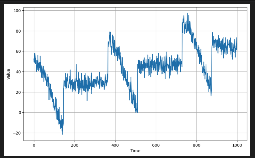
# Plot the validation set
plot_series(time_valid, x_valid)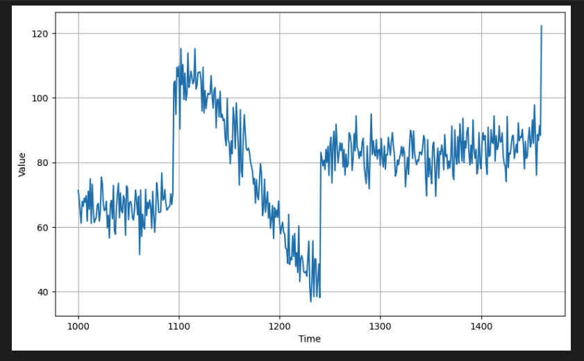
[4] Prepare features and labels
- 이제 데이터 window를 준비한다. 원하는 경우 나중에 쉽게 조정할 수 있도록 별도의 셀에 매개변수를 선언하는 것이 좋다.
모듈식으로 만들어 필요한 경우 다른 프로젝트에서 쉽게 사용할 수 있다.
 def windowed_dataset(series, window_size, batch_size, shuffle_buffer):
    """Generates dataset windows

    Args:
      series (array of float) - contains the values of the time series
      window_size (int) - the number of time steps to include in the feature
      batch_size (int) - the batch size
      shuffle_buffer(int) - buffer size to use for the shuffle method

    Returns:
      dataset (TF Dataset) - TF Dataset containing time windows
    """

    # Generate a TF Dataset from the series values
    dataset = tf.data.Dataset.from_tensor_slices(series)

    # Window the data but only take those with the specified size
    dataset = dataset.window(window_size + 1, shift=1, drop_remainder=True)

    # Flatten the windows by putting its elements in a single batch
    dataset = dataset.flat_map(lambda window: window.batch(window_size + 1))

    # Create tuples with features and labels
    dataset = dataset.map(lambda window: (window[:-1], window[-1]))

    # Shuffle the windows
    dataset = dataset.shuffle(shuffle_buffer)

    # Create batches of windows
    dataset = dataset.batch(batch_size).prefetch(1)

return dataset- 여기서는 데이터 세트.window()를 호출할 때 window_size + 1을 지정했는데, 다음 포인트를 레이블로 사용하고 있음을 나타내는 +1이다.
예를 들어 처음 20개의 포인트가 피처가 되고 21번째 포인트가 레이블이 될 것이다.
# Parameters
window_size = 20
batch_size = 32
shuffle_buffer_size = 1000

dataset = windowed_dataset(x_train, window_size, batch_size, shuffle_buffer_size)
이제 훈련 세트에서 데이터 세트 window를 생성할 수 있다.
# Print properties of a single batch
for windows in dataset.take(1):
  print(f'data type: {type(windows)}')
  print(f'number of elements in the tuple: {len(windows)}')
  print(f'shape of first element: {windows[0].shape}')
  print(f'shape of second element: {windows[1].shape}')

# output
data type: <class 'tuple'>
number of elements in the tuple: 2
shape of first element: (32, 20)
shape of second element: (32,)
2024-04-18 10:01:44.540294: W tensorflow/core/framework/local_rendezvous.cc:404] Local rendezvous is aborting with status: OUT_OF_RANGE: End of sequence
출력을 통해서 함수가 예상대로 작동하는지 확인한다.
tf.data.Dataset API의 take() 메소드를 사해 단일 배치를 가져와서, 해당 요소의 데이터 유형 및 모양과 같은 이 배치의 여러 속성을 프린트해본다.
예상한 대로 2요소 튜플(예: (리처, 레이블))이 있어야 하며 이들의 모양은 이전에 선언한 배치 및 창 크기(기본적으로 각각 32 및 20)와 일치해야 한다.
[5] Build and compile the model
- 이제 단일 계층 신경망을 구축한다. 단일 단위의 Dense 레이어를 쌓고 나get_weights() 메서드를 사용하여 최종 가중치를 볼 수도 있도록 레이어를 변수 l0에 할당한다.
l0 = tf.keras.layers.Dense(units=1, input_shape=[window_size])
model = tf.keras.models.Sequential([l0]

model.compile(loss='mse', optimizer=tf.keras.optimizers.SGD(momentum=0.9, learning_rate=1e-6))

print(f"Layer weights : {l0.get_weights()}")


model.summary()

# output
Layer wieghts : [array([[-0.06430715],
       [-0.43933353],
       [ 0.0349232 ],
       [-0.30867416],
       [-0.28906775],
       [ 0.16387522],
       [ 0.03538144],
       [-0.14311546],
       [ 0.1772303 ],
       [ 0.03114396],
       [-0.48953128],
       [-0.0481953 ],
       [ 0.42053586],
       [-0.26347485],
       [-0.26953095],
       [ 0.42382163],
       [ 0.2824847 ],
       [-0.16823238],
       [ 0.19963837],
       [-0.0442909 ]], dtype=float32), array([0.], dtype=float32)]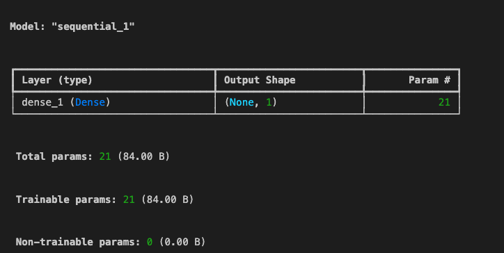
- 평균 제곱 오차(mse)를 손실 함수로 설정하고 확률적 경사하강법(SGD)을 사용하여 훈련 중에 가중치를 최적화한다.
[6] Train the Model
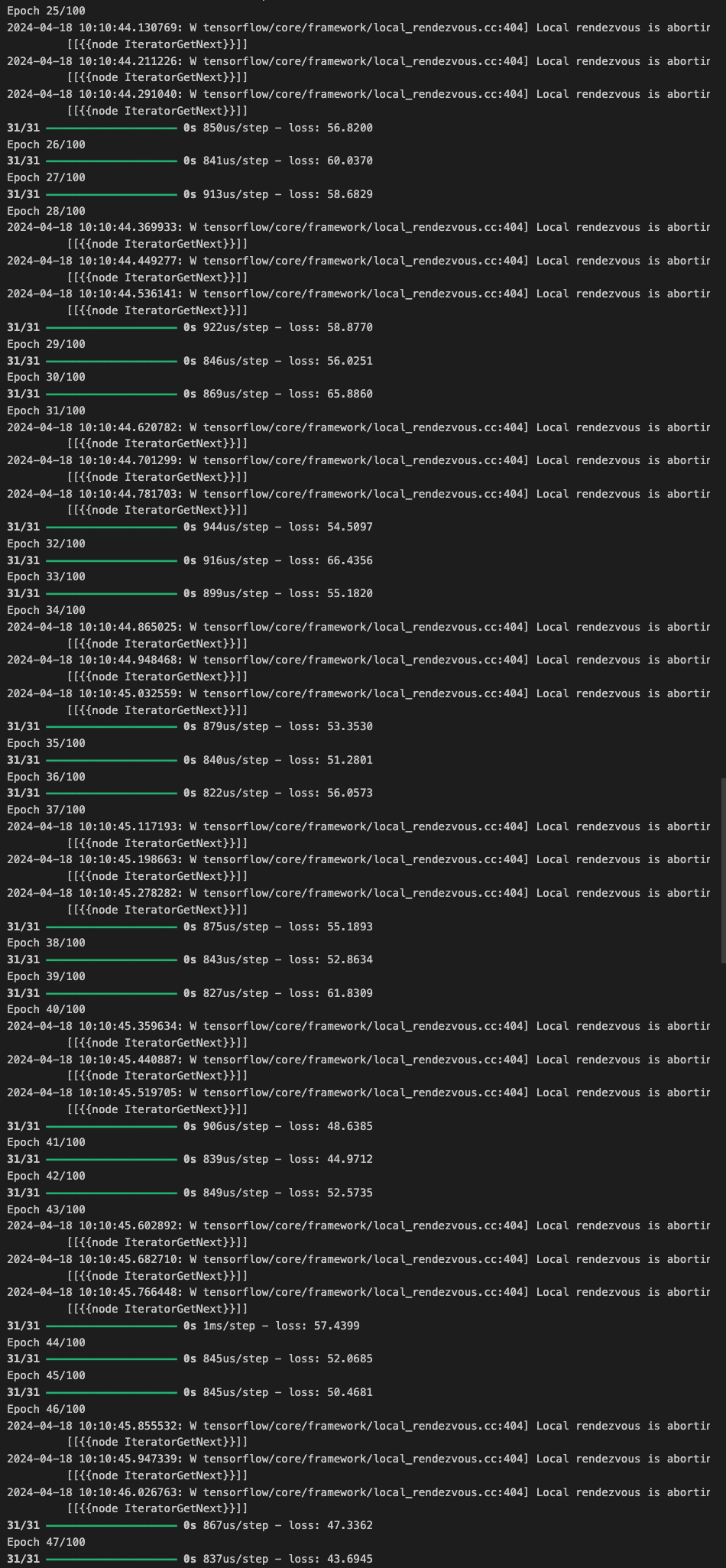
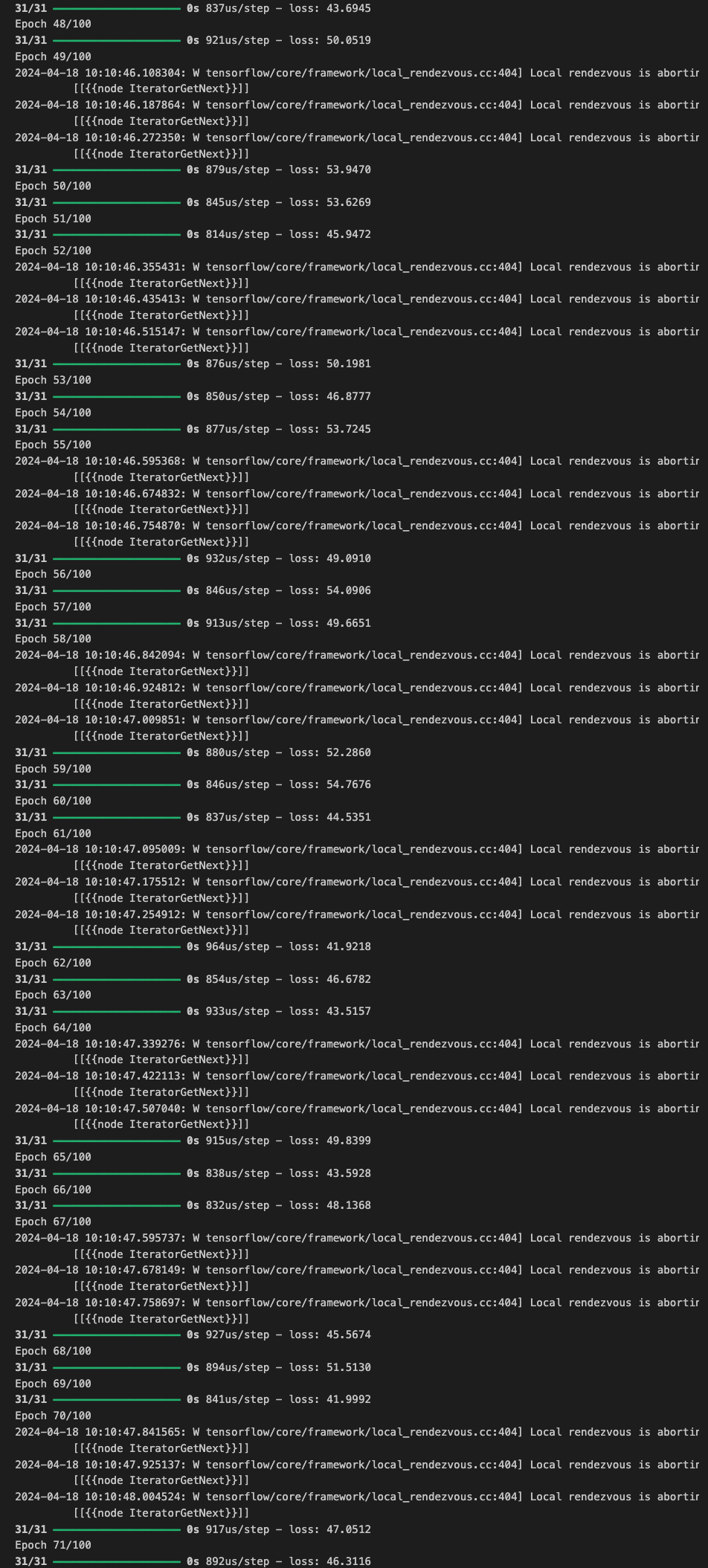
이제 모델 학습을 진행하기 위해 준비된 데이터로 100 epoch 동안 학습을 진행한다.
history = model.fit(dataset, epochs=100)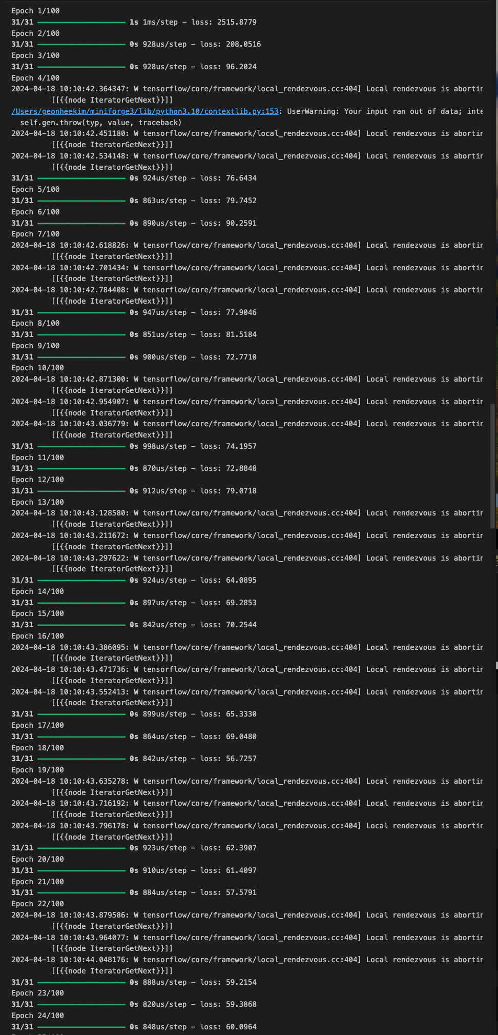

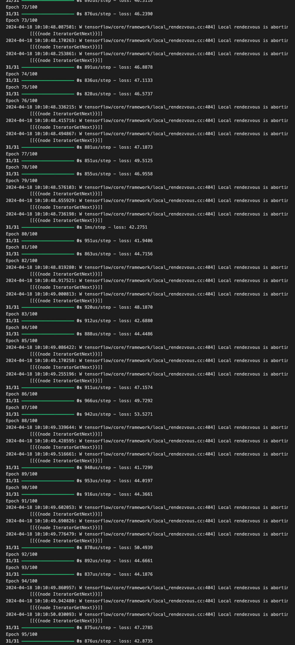
get_weights() 메서드를 다시 호출하면 최종 가중치를 볼 수 있다.
print(f"Layer weights -> {l0.get_weights()}")

# output
Layer weights -> [array([[-1.49012934e-02],
       [-5.41206449e-02],
       [ 7.94099048e-02],
       [-3.35199684e-02],
       [-3.66221159e-03],
       [ 3.79930586e-02],
       [-7.20266835e-05],
       [-1.97986476e-02],
       [ 3.43745314e-02],
       [ 3.04847732e-02],
       [-8.96111652e-02],
       [-2.18748581e-04],
       [ 5.89985587e-02],
       [-1.62686165e-02],
       [-4.22310904e-02],
       [ 1.18681304e-01],
       [ 7.76400790e-02],
       [ 1.20957568e-01],
       [ 2.88641304e-01],
       [ 4.29465711e-01]], dtype=float32), array([0.0168612], dtype=float32)]
[7] model prediction
- 학습이 완료되면 이제 모델의 성능을 측정한다. 일련의 window 데이터를 전달해 모델 예측을 생성할 수 있다. 원래 계열 배열에서 window을 분할하려는 경우 이를 모델에 전달하기 전에 배치 차원을 추가해야 한다. 이는 np.newaxis 상수로 인덱싱하거나 np.expand_dims() 메소드를 사용하여 수행할 수 있다.
series[0:20]

# output
array([52.48357 , 49.35275 , 53.314735, 57.711823, 48.934444, 48.931244,
       57.982895, 53.897125, 47.67393 , 52.68371 , 47.591717, 47.506374,
       50.959415, 40.086178, 40.919415, 46.612473, 44.228207, 50.720642,
44.454983, 41.76799 ], dtype=float32)series[0:20][np.newaxis]
# output
array([[52.48357 , 49.35275 , 53.314735, 57.711823, 48.934444, 48.931244,
57.982895, 53.897125, 47.67393 , 52.68371 , 47.591717, 47.506374,
50.959415, 40.086178, 40.919415, 46.612473, 44.228207, 50.720642,
44.454983, 41.76799 ]], dtype=float32)np.expand_dims(series[0:20], axis=0)
# output
array([[52.48357 , 49.35275 , 53.314735, 57.711823, 48.934444, 48.931244,
57.982895, 53.897125, 47.67393 , 52.68371 , 47.591717, 47.506374,
50.959415, 40.086178, 40.919415, 46.612473, 44.228207, 50.720642,
44.454983, 41.76799 ]], dtype=float32)# Shape of the first 20 data points slice
print(f'shape of series[0:20]: {series[0:20].shape}')
# Shape after adding a batch dimension
print(f'shape of series[0:20][np.newaxis]: {series[0:20][np.newaxis].shape}')
# Shape after adding a batch dimension (alternate way)
print(f'shape of series[0:20][np.newaxis]: {np.expand_dims(series[0:20], axis=0).shape}')
# Sample model prediction
print(f'model prediction: {model.predict(series[0:20][np.newaxis])}')
# output
shape of series[0:20]: (20,)
shape of series[0:20][np.newaxis]: (1, 20)
shape of series[0:20][np.newaxis]: (1, 20)
1/1 ━━━━━━━━━━━━━━━━━━━━ 0s 28ms/step
model prediction: [[44.937992]]- 측정항목을 계산하려면 검증 세트에 대한 모델 예측을 생성해야 한다.
이 세트는 전체 시리즈의 인덱스 1000~1460에 있는 포인트를 참조한다.
모델에서 해당 단계를 생성하려면 단계를 코딩해야 한다.
기본적으로 전체 계열을 한 번에 20포인트씩 모델에 공급하고 모든 결과를 예측 목록에 추가한다. 그런 다음 검증 세트에 해당하는 포인트를 분할한다.
# Initialize a list
forecast = []

# Use the model to predict data points per window size
for time in range(len(series) - window_size):
  forecast.append(model.predict(series[time:time + window_size][np.newaxis]))

# Slice the points that are aligned with the validation set
forecast = forecast[split_time - window_size:]

# Compare number of elements in the predictions and the validation set
print(f'length of the forecast list: {len(forecast)}')
print(f'shape of the validation set: {x_valid.shape}')

# output
length of the forecast list: 461
shape of the validation set: (461,)
아래의 슬라이스 인덱스는 Split_time - window_size인데, 예측 목록이 계열보다 20포인트(즉, window 크기)만큼 작기 때문이다. window 크기가 20이므로 예측 목록의 첫 번째 데이터 포인트는 인덱스 20의 시간에 대한 예측에 해당한다. 인덱스 0~19는 창 크기보다 작기 때문에 예측을 할 수 없다. 따라서 Split_time - window_size:로 분할하면 검증 세트의 시간 인덱스와 일치하는 시간 인덱스의 포인트를 얻게 된다.
결과를 시각화하려면 예측을 plot_series() 유틸리티 함수가 허용하는 형식으로 변환한다. 여기에는 배열을 numpy 배열로 변환하고 1차원 축을 삭제하면 된다.
# Preview shapes after using the conversion and squeeze methods
print(f'shape after converting to numpy array: {np.array(forecast).shape}')
print(f'shape after squeezing: {np.array(forecast).squeeze().shape}')

# Convert to a numpy array and drop single dimensional axes
results = np.array(forecast).squeeze()

# Overlay the results with the validation set
plot_series(time_valid, (x_valid, results))

# outout
shape after converting to numpy array: (461, 1, 1)
shape after squeezing: (461,)
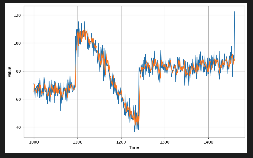
이전과 동일한 함수를 호출하여 측정항목을 계산할 수 있다.
현재 MAE는 5에 가깝다.
# Compute the metrics
print(tf.keras.metrics.mean_squared_error(x_valid, results).numpy())
print(tf.keras.metrics.mean_absolute_error(x_valid, results).numpy())

# output
45.70831
5.035314
여기서는 시계열 데이터를 기반으로 단일 계층 신경망을 구축하고 학습했다. window 데이터를 준비하여 모델에 제공하면 최종 예측은 1주차에 수행한 통계 분석과 비슷한 결과를 보여준다. 다음은 더 많은 레이어를 추가하고 다음과 같은 경우에 수행할 수 있는 몇 가지 최적화를 반영하여 모델을 학습시켜보도록 한다.