[Tensorflow] 4. Sequences, Time Series and Prediction(2. Deep Neural Networks for Time Series) : programminig (3)

[Tensorflow] 4. Sequences, Time Series and Prediction(2. Deep Neural Networks for Time Series) : programminig (3)

Training a Deep Neural Network with Time Series Data(시계열 데이터를 사용한 심층 신경망 훈련)

• 이전에는 레이어를 1개로 한 단층 레이어를 사용했지만 여기서는 시계열 데이터를 사용해 딥러닝에 Dense 레이어를 추가한다.
  추가로 가중치가 더 빠르게 수렴되도록 모델의 학습 속도를 조정하는 기술을 적용해본다. 이는 학습 전에 학습률을 추측할 수 있다.

[1] import & Utilities

import tensorflow as tf
import numpy as np
import matplotlib.pyplot as plt

def plot_series(time, series, format="-", start=0, end=None):
    """
    Visualizes time series data

    Args:
      time (array of int) - contains the time steps
      series (array of int) - contains the measurements for each time step
      format - line style when plotting the graph
      label - tag for the line
      start - first time step to plot
      end - last time step to plot
    """

    # Setup dimensions of the graph figure
    plt.figure(figsize=(10, 6))
    
    if type(series) is tuple:

      for series_num in series:
        # Plot the time series data
        plt.plot(time[start:end], series_num[start:end], format)

    else:
      # Plot the time series data
      plt.plot(time[start:end], series[start:end], format)

    # Label the x-axis
    plt.xlabel("Time")

    # Label the y-axis
    plt.ylabel("Value")

    # Overlay a grid on the graph
    plt.grid(True)

    # Draw the graph on screen
    plt.show()

def trend(time, slope=0):
    """
    Generates synthetic data that follows a straight line given a slope value.

    Args:
      time (array of int) - contains the time steps
      slope (float) - determines the direction and steepness of the line

    Returns:
      series (array of float) - measurements that follow a straight line
    """

    # Compute the linear series given the slope
    series = slope * time

    return series

def seasonal_pattern(season_time):
    """
    Just an arbitrary pattern, you can change it if you wish
    
    Args:
      season_time (array of float) - contains the measurements per time step

    Returns:
      data_pattern (array of float) -  contains revised measurement values according 
                                  to the defined pattern
    """

    # Generate the values using an arbitrary pattern
    data_pattern = np.where(season_time < 0.4,
                    np.cos(season_time * 2 * np.pi),
                    1 / np.exp(3 * season_time))
    
    return data_pattern

def seasonality(time, period, amplitude=1, phase=0):
    """
    Repeats the same pattern at each period

    Args:
      time (array of int) - contains the time steps
      period (int) - number of time steps before the pattern repeats
      amplitude (int) - peak measured value in a period
      phase (int) - number of time steps to shift the measured values

    Returns:
      data_pattern (array of float) - seasonal data scaled by the defined amplitude
    """
    
    # Define the measured values per period
    season_time = ((time + phase) % period) / period

    # Generates the seasonal data scaled by the defined amplitude
    data_pattern = amplitude * seasonal_pattern(season_time)

    return data_pattern

def noise(time, noise_level=1, seed=None):
    """Generates a normally distributed noisy signal

    Args:
      time (array of int) - contains the time steps
      noise_level (float) - scaling factor for the generated signal
      seed (int) - number generator seed for repeatability

    Returns:
      noise (array of float) - the noisy signal
    """

    # Initialize the random number generator
    rnd = np.random.RandomState(seed)

    # Generate a random number for each time step and scale by the noise level
    noise = rnd.randn(len(time)) * noise_level
    
    return noise

[2] Generate the Dataset & Split the Dataset

# Parameters
time = np.arange(4 * 365 + 1, dtype="float32")
baseline = 10
amplitude = 40
slope = 0.05
noise_level = 5

# Create the series
series = baseline + trend(time, slope) + seasonality(time, period=365, amplitude=amplitude)

# Update with noise
series += noise(time, noise_level, seed=42)

# Plot the results
plot_series(time, series)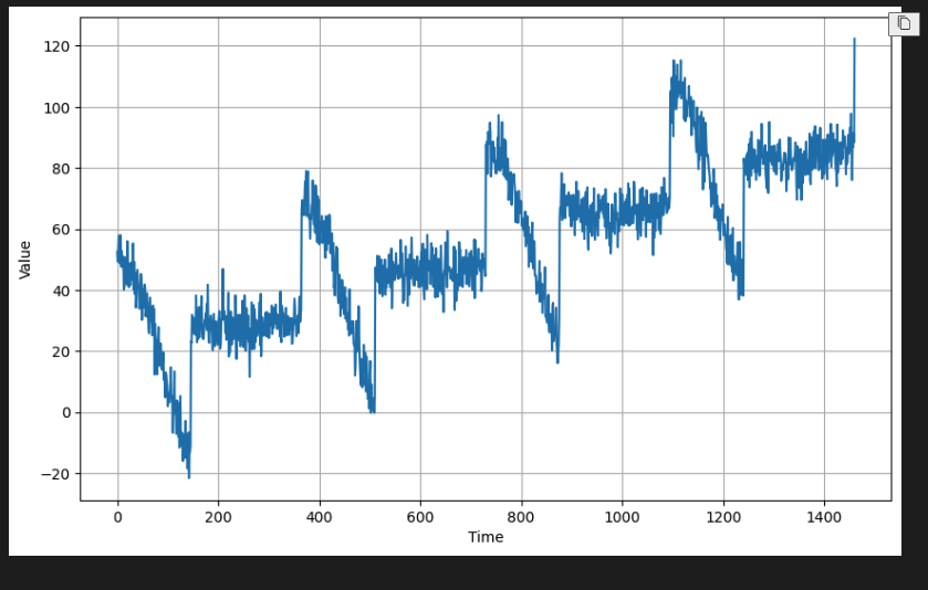

split_time =1000

time_train = time[:split_time]
x_train = series[:split_time]

time_valid = time[split_time:]
x_valid = series[split_time:]

[3] `Prepare Features and Labels

def windowed_dataset(series, window_size, batch_size, buffer_size):
    
    dataset = tf.data.Dataset.from_tensor_slices(series)
    dataset = dataset.window(window_size+1, shift=1, drop_remainder=True)
    dataset = dataset.flat_map(lambda window : window.batch(window_size+1))
    dataset = dataset.map(lambda window : (window[:-1], window[-1]))
    dataset = dataset.shuffle(buffer_size)
    dataset = dataset.batch(batch_size).prefetch(1)
    
    return dataset

여기서는 윈도우 사이즈를 20, 배치를 32, 셔플 하이퍼파라미터를 1000으로 지정했다.

window_size = 20
batch_size = 32
shuffle_buffer_size =1000

dataset = windowed_dataset(x_train, window_size, batch_size, shuffle_buffer_size)
dataset

#output
<_PrefetchDataset element_spec=(TensorSpec(shape=(None, None), dtype=tf.float32, name=None), TensorSpec(shape=(None,), dtype=tf.float32, name=None))>

[4] Build the model

model_baseline = tf.keras.models.Sequential([
    tf.keras.layers.Dense(10, activation='relu', input_shape=[window_size]),
    tf.keras.layers.Dense(10, activation='relu'),
    tf.keras.layers.Dense(1)
])

model_baseline.compile(loss='mse',
                       optimizer = tf.keras.optimizers.SGD(learning_rate=1e-6,
                                                           momentum=0.9))
                                                           
model_baseline.summary()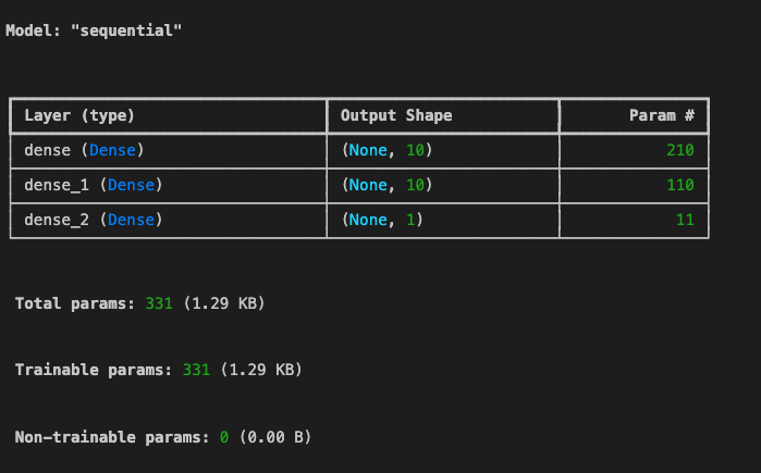

[5] Train the model

model_baseline.fit(dataset, epochs=100)

• 이제 학습한 모델에 몇 가지 예측을 얻고 이전과 같이 시각화한다.
  신경망이 더 깊기 때문에 예측 속도가 느려질 수 있으므로 불필요한 계산을 최소화하는 것이 좋.

• 이전 실습에서는 전체 계열 데이터를 사용하여 예측을 생성했었다.
  결과적으로 예측 목록에 1,441개의 포인트가 생성되었으며, Forecast = Forecast[split_time - window_size:]를 사용하여 검증 세트와 일치하는 461개의 포인트를 분할했다.

• 처음부터 461개의 포인트를 생성하면 이 프로세스를 더 빠르게 만들 수 있고, 이렇게 하면 나중에 버려질 포인트를 예측하는 데 시간을 낭비하지 않아도 된다. predict() 메서드를 호출하기 전에 원래 계열에서 필요한 포인트를 가져온다.
  이 과정에서 모든 예측은 이미 검증 세트와 일치하며 for 루프는 1,441회가 아닌 461회만 실행된다.

# Initialize a list
forecast = []

# Reduce the original series
forecast_series = series[split_time - window_size:]

# Use the model to predict data points per window size
for time in range(len(forecast_series) - window_size):
  forecast.append(model_baseline.predict(forecast_series[time:time + window_size][np.newaxis]))

# Convert to a numpy array and drop single dimensional axes
results = np.array(forecast).squeeze()

# Plot the results
plot_series(time_valid, (x_valid, results))

# Compute the metrics
print(tf.keras.metrics.mean_squared_error(x_valid, results).numpy())
print(tf.keras.metrics.mean_absolute_error(x_valid, results).numpy())

#output
50.47491
5.1362295

[6] Tune the learning rate

• 선택한 초기 학습률(예: 1e-6)로 훈련이 잘 진행되는 것을 확인했다. 그러나 이 설정이 이 특정 모델에 가장 적합한 설정인지는 아직 확실하지 않다. 더 복잡한 모델이 있는 경우에는 학습 속도를 조정하는 데 시간을 투자하면 더 나은 훈련 결과를 얻을 수 있다.

• 학습률을 조정하는 방법에 대해서 진행하기 위해 먼저 위에서 학습한 동일한 모델 아키텍처를 만든다.

model_tune = tf.keras.models.Sequential([
    tf.keras.layers.Dense(10, input_shape=[window_size], activation='relu'),
    tf.keras.layers.Dense(10, activation='relu'),
    tf.keras.layers.Dense(1)
])

학습률 스케줄러 콜백(LearningRateScheduler)을 선언한다. 이를 통해 훈련 중 에포크 번호를 기반으로 학습 속도를 동적으로 설정할 수 있다.
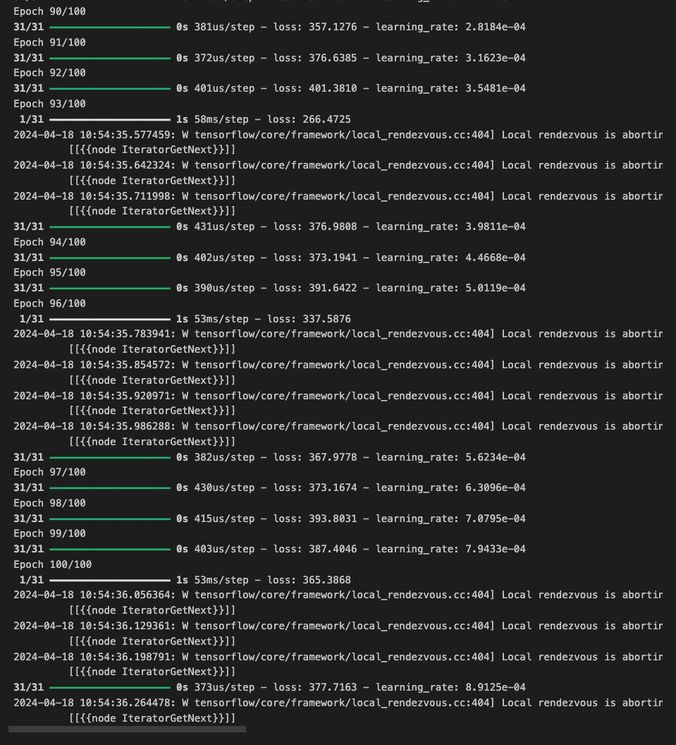
아래와 같이 학습률 값을 선언하는 람다 함수를 전달하는데, epoch 0의 1e-8에서 시작하고 훈련이 진행됨에 따라 10**(epoch / 20)만큼 확장된다.

lr_scheduler = tf.keras.callbacks.LearningRateScheduler(lambda epoch: 1e-8*10**(epoch/20))

그런 다음 모델을 컴파일한다.
여기서는 옵티마이저의 learning_rate 인수를 설정할 필요가 없다. 기본값(예: SGD의 경우 0.01)을 그대로 두고 학습률 스케줄러가 이를 동적으로 설정하도록 허용할 수 있다.

# Initialize the optimizer
optimizer = tf.keras.optimizers.SGD(momentum=0.9)

# Set the training parameters
model_tune.compile(loss="mse", optimizer=optimizer)

fit() 메서드의 콜백 매개변수에 lr_schedule 콜백을 전달한다.
학습을 행하면 콘솔 출력에서 lr로 표시된 특정 에포크의 학습률을 볼 수 있다. 사용한 람다 함수에 따라 예상대로 증가할 것이다.

history = model_tune.fit(dataset, epochs=100, callbacks=[lr_scheduler])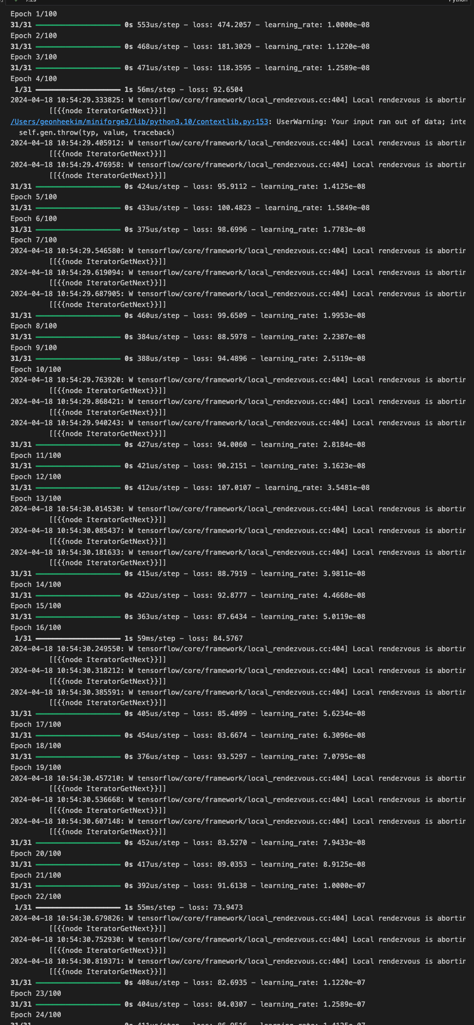

다음은 훈련 결과를 플로팅했고, 학습률의 각 값에서 손실을 시각화해본다.

# Define the learning rate array
lrs = 1e-8 * (10 ** (np.arange(100) / 20))

# Set the figure size
plt.figure(figsize=(10, 6))

# Set the grid
plt.grid(True)

# Plot the loss in log scale
plt.semilogx(lrs, history.history["loss"])

# Increase the tickmarks size
plt.tick_params('both', length=10, width=1, which='both')

# Set the plot boundaries
plt.axis([1e-8, 1e-3, 0, 300])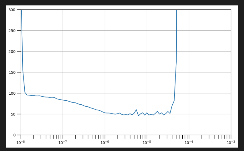

• 위에 생성된 그래프는 손실을 낮추는 학습률 범위(즉, 아래쪽으로 기울어짐)와 훈련을 불안정하게 만드는 학습률 범위(예: 들쭉날쭉한 가장자리 및 위쪽을 향함)의 값을 보여준다.
  일반적으로 하향 경사에서 한 점을 선택하는 것이 좋은데, 이는 신경망이 해당 시점에서 여전히 학습 중이고 안정적이라는 것을 의미한다.
  그래프의 최소 지점에 가까운 것을 선택하면 다음 셀에 표시되는 것처럼 훈련이 해당 손실 값으로 더 빠르게 수렴된다.

위에서 확인한 손실을 낮추는 학습률 범위를 세팅하기 위해 먼저 동일한 모델 아키텍처를 다시 초기화한다.

# Build the model
model_tune = tf.keras.models.Sequential([
  tf.keras.layers.Dense(10, activation="relu", input_shape=[window_size]),
  tf.keras.layers.Dense(10, activation="relu"),
  tf.keras.layers.Dense(1)
])

그런 다음 최소값에 가까운 학습률로 최적화 파라미터를 선택한다.
위 그래프에 따라서 10^-6을 선택했다.

그런 다음 이전과 같이 모델을 컴파일하고 학습할 수 있다. 손실 값을 관찰하고 이를 이전에 가지고 있던 기준 모델의 출력과 비교한다.

model.compile(loss='mse',
              optimizer=tf.keras.optimizers.SGD(momentum=0.9, learning_rate=1e-6))

history = model.fit(dataset, epochs=100)

# Plot the loss
loss = history.history['loss']
epochs = range(len(loss))
plt.plot(epochs, loss, 'b', label='Training Loss')
plt.show()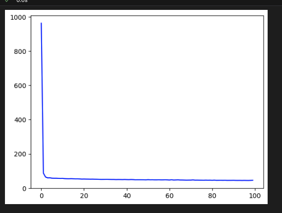

fit() 메서드에서 반환된 History 객체에서 손실 값을 가져와서 표시할 수 있다. 보시다시피, 훈련 후에도 모델은 여전히 하향 추세를 보이고 있다.

# Plot all but the first 10
loss = history.history['loss']
epochs = range(10, len(loss))
plot_loss = loss[10:]
plt.plot(epochs, plot_loss, 'b', label='Training Loss')
plt.show()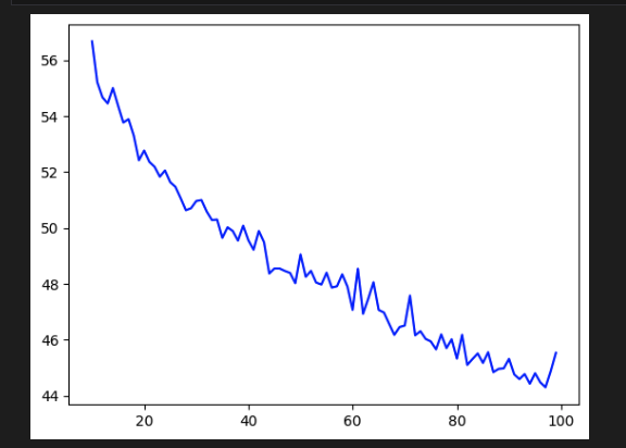

예측을 다시 가져와 검증 세트에 오버레이할 수 있다.

forecast = []

forecast_series = series[split_time-window_size:]

for time in range(len(forecast_series)-window_size):
    forecast.append(model.predict(forecast_series[time:time+window_size][np.newaxis]))

results = np.array(forecast).squeeze()

plot_series(time_valid, (x_valid, results))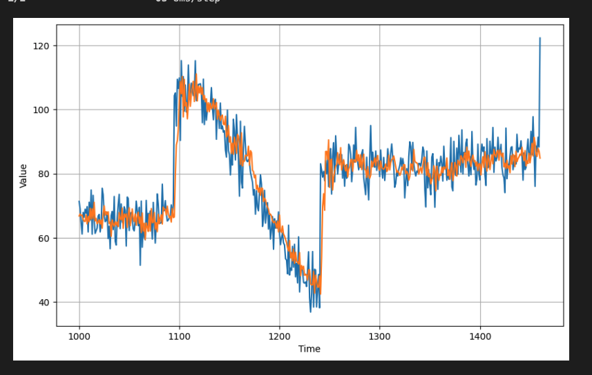

마지막으로 지표를 계산할 수 있으며 기준선과 비교하여 유사한 수치에 도달해야 한다. 상황이 훨씬 더 나쁘다면 모델이 과적합되었을 수 있으므로 이를 방지하기 위해 알고 있는 기술을 사용할 수 있다.(예: 드롭아웃 추가).

print(tf.keras.metrics.mean_squared_error(x_valid, results).numpy())
print(tf.keras.metrics.mean_absolute_error(x_valid, results).numpy())

# output
47.749836
5.098338

이러한 과정을 통해 예측을 위해 심층 신경망을 사용했다. 그 과정에서 특히 학습률에 관해 초매개변수 조정을 수행했다