앞선 iris data 분류 1에서 이어지는 내용이다.
마지막에 Accuracy를 확인했을 때 매우 높은 수치가 측정됐다.
과연 그 수치가 맞다고 할 수 있을까?
알 수 없으니 더 자세히 들여다봐야 한다.
📚 데이터 분류 확인
만든 Decision Tree 모델이 iris 품종을 분류하기 위해 데이터를 어떻게 나눴는지 확인해보자.
그 전에 한 가지 추가로 설치하고 진행한다.
pip install mlxtend
from mlxtend.plotting import plot_decision_regions

plt.figure(figsize=(14,8))
plot_decision_regions(X=iris.data[:, 2:], y=iris.target, clf=iris_tree, legend=2)
plt.show()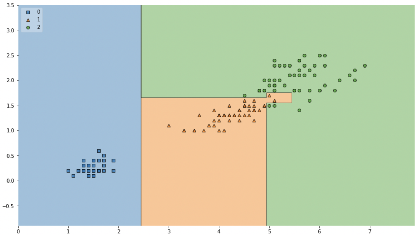
결과 이미지는 다를 수 있다.
이유는 결정트리가 랜덤성을 갖고 있기 때문이다.
💡 이제 결정 경계를 보고 판단을 해야한다.
- 경계면이 올바른 것일까?
- 이 결과는 내가 가진 데이터를 벗어나 일반화 될 수 있을까?
내가 가진 데이터는 유한하고, 이를 이용해서 일반화를 추구하게 되는데
이때 복잡한 경계면은 모델의 성능을 결국 나쁘게 만든다.
즉, 오버피팅을 주의해야 한다.
📚 데이터 분리
iris에 대한 새로운 데이터를 확보할 수 없으니 갖고 있는 데이터를 훈련 검증 평가 로 분리해 모델을 학습시키고 테스트한다.
여기서 각 클래스별로 고르게 데이터를 분리하기 위해 stratify 옵션을 쓸 것이다.
👉 훈련/테스트 데이터로 분리
from sklearn.model_selection import train_test_split

features = iris.data[:, 2:]
labels = iris.target

X_train, X_test, y_train, y_test = train_test_split(features, labels,
						    test_size=0.2,
                                   		    stratify=labels,
                                  		    random_state=13)
지금 내가 분리한 데이터의 각 클래스별 갯수를 확인하고 싶을 때 아래 코드를 활용할 수 있다.
np.unique(y_test, return_counts=True)📚 결정나무 모델 구현
다시 train 데이터만 대상으로 결정나무 모델을 만들어보자
- 학습의 일관성을 위해 random_state 고정
- 모델 단순화를 위해 max_depth 조정
iris_tree = DecisionTreeClassifier(max_depth=2, random_state=13)
iris_tree.fit(X_train, y_train)
👉 train 데이터에 대한 Accuracy 확인
y_pred_tr = iris_tree.predict(X_train)
accuracy_score(y_train, y_pred_tr)
📚 모델 확인
내가 구현한 모델이 어떤 기준으로 분류가 되었는지를 트리 형태로 볼 수 있다.
from sklearn import tree

tree.plot_tree(iris_tree, feature_names = iris.feature_names,
	     rounded=True, filled=True)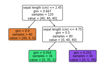
👉 훈련데이터에 대한 결정경계 확인
plt.figure(figsize=(12,8))
plot_decision_regions(X=X_train, y=y_train, clf=iris_tree, legend=2)
plt.show()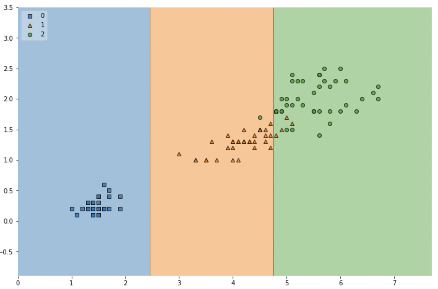
위에서와 다르게 조금 더 단순한 결정경계가 생긴 것을 볼 수 있다.
👉 test data에 대한 Accuracy 확인
y_pred_test = iris_tree.predict(X_test)
accuracy_score(y_test, y_pred_test)
📚 전체 데이터 관찰
scatter_highlight_kwargs = {'s':150, 'label':'Test data', 'alpha':0.9}
scatter_kwargs = {'s':120, 'edgecolor':None, 'alpha':0.7}

plt.figure(figsize=(12,8))
plot_decision_regions(X=features, y=labels,
                     X_highlight=X_test, clf=iris_tree, legend=2,
                     scatter_highlight_kwargs=scatter_highlight_kwargs,
                     scatter_kwargs=scatter_kwargs,
                     contourf_kwargs={'alpha':0.2})
plt.show()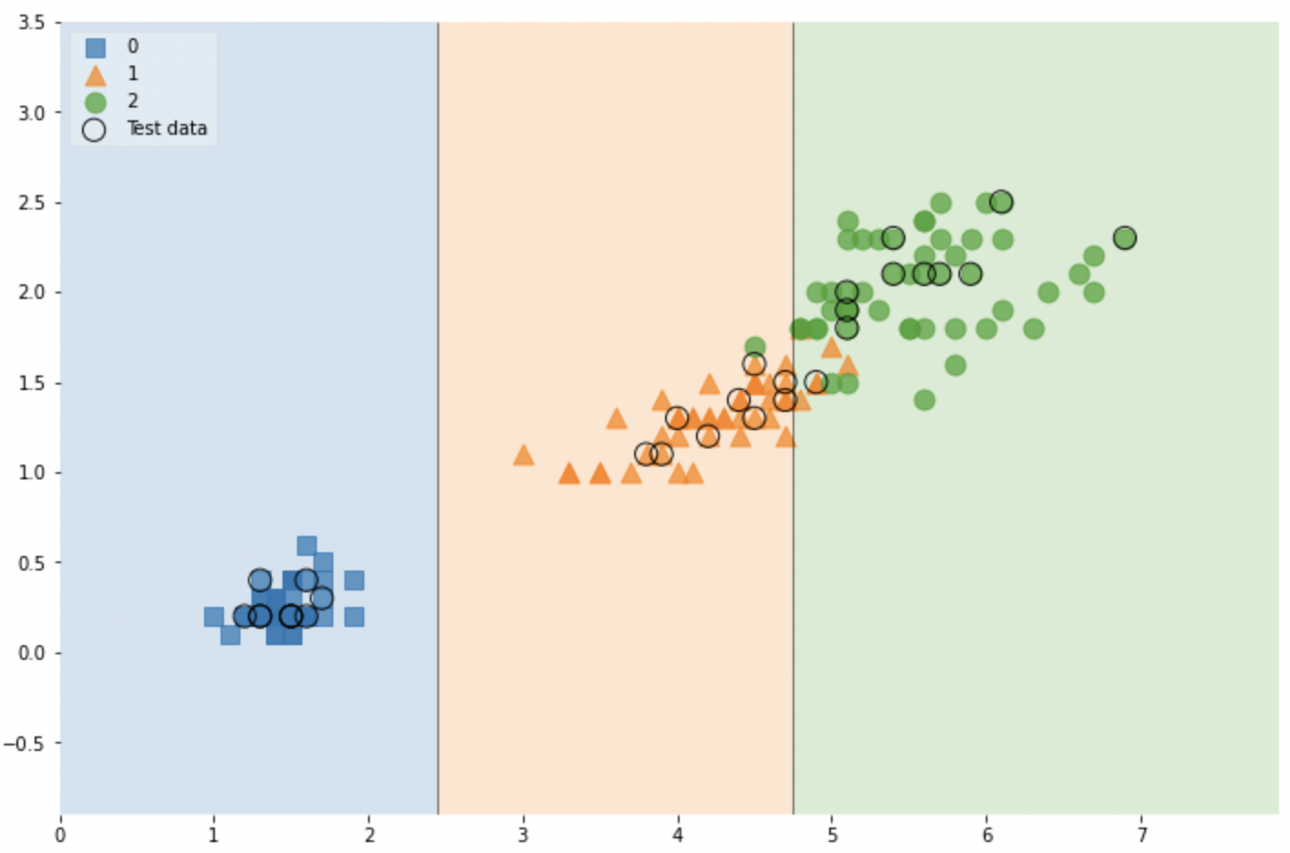
👉 feature를 4개를 줘본다
features = iris.data
labels = iris.target

X_train, X_test, y_train, y_test = train_test_split(features, labels,
                                                   test_size=0.2,
                                                   stratify=labels,
                                                   random_state=13)
iris_tree = DecisionTreeClassifier(max_depth=2, random_state=13)
iris_tree.fit(X_train, y_train)

tree.plot_tree(iris_tree, feature_names = iris.feature_names, rounded=True, filled=True);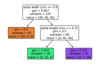
📚 모델 사용
길 가다가 주운 iris가 sepal과 petal의 length, width가 각각 [4.3, 2. , 1.2, 1.0] 이라면 아래와 같이 할 수 있다.
test_data = [4.3, 2. , 1.2, 1.0]
iris_tree.predict_proba(test_data)
👉 속성들의 중요도를 나타내자
iris_clf_model = dict(zip(iris.feature_names, iris_tree.feature_importances_))