End to End 머신러닝 프로젝트

• 큰 그림을 봅니다
• 데이터를 구합니다
• 데이터로부터 통찰을 얻기 위해 탐색하고 시각화 합니다
• 머신러닝 알고리즘을 위해 데이터를 준비 합니다
• 모델을 선택하고 훈련시킵니다
• 모델을 상세하게 조정합니다
• 솔루션을 제시합니다
• 시스템을 론칭하고 모니터링하고 유지 보수 합니다.

머신러닝 프로젝트를 할 때 큰 그림을 보지 않고 주먹 구구 식으로 프로젝트 했던 경험이 있다.
이때의 비효율성과 내가 왜?이걸 하고 있지 라는 생각은 정말 작업효율과 흥미 모두 떨어지게 한다.
큰그림을 보자

테스트 데이터 셋 만들기

numpy permutation으로 구하기

import numpy as np

# For illustration only. Sklearn has train_test_split()
def split_train_test(data, test_ratio):
    shuffled_indices = np.random.permutation(len(data))
    test_set_size = int(len(data) * test_ratio)
    test_indices = shuffled_indices[:test_set_size]
    train_indices = shuffled_indices[test_set_size:]
    return data.iloc[train_indices], data.iloc[test_indices]

• 위방법의 문제점은 데이터가 계속 변경 될 수 있음
• 그래서 각 샘플의 식별자identifier를 사용해서 분할 하자

식별자를 활용해 분할

from zlib import crc32

def test_set_check(identifier, test_ratio):
    return crc32(np.int64(identifier)) & 0xffffffff < test_ratio * 2**32 #crc32 해쉬함수 이용 
#0xfffffffff  - > 2**32 -1   identifier 가 들어오면 test인지  아닌지  

def split_train_test_by_id(data, test_ratio, id_column):
    ids = data[id_column]
    in_test_set = ids.apply(lambda id_: test_set_check(id_, test_ratio))
    return data.loc[~in_test_set], data.loc[in_test_set]

• 위 방법 역시 만약 나중에 db업데이트가 되어 수정되거나 삭제되면 행 번호가 갱신 되지 않을수가 있음
• id를 만드는데 안전한 feature들을 사용해야함

유니크한 id를 사용해서 테스트셋 구현

housing_with_id["id"] = housing["longitude"] * 1000 + housing["latitude"] #지역은 유니크하게 경도위도 속성활용
train_set, test_set = split_train_test_by_id(housing_with_id, 0.2, "id") 

scikit-Learn 에서 기본적으로 제공되는 데이터 분할 함수 활용

import sklearn
from sklearn.model_selection import train_test_split

train_set, test_set = train_test_split(housing, test_size=0.2, random_state=42)

계층적 샘플링

• 전체 데이터를 계층(strata)라는 같은 급의 그룹으로 나누다.
• 그리고 테스트 데이터가 전체 데이터를 잘 대표 할 수 있게 원래의 분포와 비슷하게 각 계층에서 올바른 수의 샘플을 추출한다

예시

housing["median_income"].hist() #모든 특성을 다 그렇게 하긴 어렵기에 가장 중요한 특성을 갖고 함

• pd.cut 함수를 활용해 위의 데이터를 binning(구간화) 해준다.

housing["income_cat"] = pd.cut(housing["median_income"],
                               bins=[0., 1.5, 3.0, 4.5, 6., np.inf],
                               labels=[1, 2, 3, 4, 5]) #데이터를 보면 감을 잡을수 이씀;; 적절하게 나눠지도록 빈만들어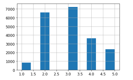

계층화 구현 코드

• sklearn을 이용하여 계층화 샘플링을한다

from sklearn.model_selection import StratifiedShuffleSplit #이미 사이킷런이 다 갖고있음 구현해주면됨

split = StratifiedShuffleSplit(n_splits=1, test_size=0.2, random_state=42)
for train_index, test_index in split.split(housing, housing["income_cat"]):
    strat_train_set = housing.loc[train_index]
    strat_test_set = housing.loc[test_index]

계층화로 샘플링한것과 그냥 샘플링 한것 차이

def income_cat_proportions(data):
    return data["income_cat"].value_counts() / len(data)

train_set, test_set = train_test_split(housing, test_size=0.2, random_state=42)

compare_props = pd.DataFrame({
    "Overall": income_cat_proportions(housing),
    "Stratified": income_cat_proportions(strat_test_set),
    "Random": income_cat_proportions(test_set),
}).sort_index()
compare_props["Rand. %error"] = 100 * compare_props["Random"] / compare_props["Overall"] - 100
compare_props["Strat. %error"] = 100 * compare_props["Stratified"] / compare_props["Overall"] - 100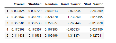

• 위 표를 보면 stratified의 경우 원래 데이터와 분포가 거의 비슷함을 알 수 있다.