[2025 CVPR] Transformers without Normalization
Abstract
(background)
- modern neural networks에서, Normalization layers는 어디서든 사용되고(unbiquitous) 필수적으로 고려되어 왔다.
(이 논문의 핵심)
- 이 연구에서는 매우 간단한 technique을 사용하여,
Transformers without normalization이 the same or better performance를 달성할 수 있음을 증명한다.
(method)
- 우리는 normalization layers in Transformers에 대해 a drop-in replacemenet로써
Dynamic Tanh (DyT), an element-wise operation 를 제안한다.
(motivation)
- DyT는 Transformers의 layer normalization이 tanh-like, S-shaped input-output mappings을 자주 만들어낸다는 관찰에 영감을 받았다.
(experiments)
-
DyT를 적용했을 때, Transformers w/o normalization은 거의 hyperparameter tuning 없이,
the performance of their normalized counterparts에 준하거나 상승했다. -
우리는 Transformers with DyT의 effective는 diverse setting에 실험했다.
recognition to generation, supervised to self-supervised learning, and computer vision to language models. -
이러한 발견은 normalization layers(NL)가 modern neural networks에서 필수적이라는 conventional understanding에 도전하며,
NL이 deep networks에서 어떤 역할을 하는지에 대한 new insights를 제공한다.
1. Introduction
(background: Normalization layer는 현대의 deep neural networks에 필수적이다. 학습을 더 빠르고 안정되게 하여 optimization을 더 잘 시킨다.)
-
2015년에 fsater and better convergence in visual recognition models을 가능하게 한 batch normalization이 제안되고부터,
many variants of normalization layers이 제안되어 왔다.
오늘날, 모든 modern networks는 normalization layers를 사용한다.
특히 dominant Transformer architectures에서는 LayerNorm, or LN이 one of the most popular한 normalizatoin layer이다. -
The widespread adoption of normalization layers는 optimization에 경험적인 benefits을 가져다줬다.
추가로 better results를 달성하기 위해, normLayer는 accelerate and stabilize convergence를 돕는다.
neural network가 wider and deeper해질수록, this necessity는 훨씬 더 중요하다.
따라서 normLayer는 deep network를 효과적으로 학습시키기 위해 매우 중요하며, 없어서는 안 될 요소로까지 여겨지고 있다.
이러한 믿음은 최근 몇 년 동안 novel architecture들이 attention or convolution layers를 대체하려는 시도는 자주 있었지만, normLayer는 거의 항상 유지되고 있다는 사실에서 은연중에 드러난다.
(proposition)
-
이 연구는 normLayer in Transformers를 대체하는 a simple alternative를 제안함으로써
normLayer가 neural network에 없어서는 안 될 필수요소라는 belief에 도전한다. -
우리의 탐구는 LN layers가 그들의 input to output을 tanh, S-shaped curves로 mapping하여,
input activations을 적절히 scaling하면서 extreme values를 눌러주는(squashing) 역할을 한다는 관찰에서 시작된다.
this insight에서 영감을 받아, 우리는 an element-wise operation termed Dynamic Tanh (DyT), defined as: , where is a learnable parameter 를 제안한다. -
DyT operation은 (1) an appropriate scaling factor 를 학습하고,
(2) the bounded tanh function를 이용해 extreme values를 눌러줌으로써
the behavior of LN을 모방(emulate)하는 것을 목표로 한다.
특히, normLayers와 달리, DyT는 activation statistics를 계산할 필요 없이 두 효과를 모두 달성한다.
(질문: 기존 normLayers들이 학습을 통해 activation의 statistics를 계산하여 normalization parameter를 학습하는 것이고,
DyT도 똑같이 학습을 통해 normalization parameter 대신 scaling factor 를 학습한다고 이해했는데,
결국 DyT도 마찬가지로 를 학습하기 위해 activation의 statistics를 계산하는 셈 아닌가?)
(AI 답변): 전통적인 LN에서는 입력 텐서가 들어올 때마다 해당 텐서에 대한 mean과 standard deviation을 계산하여 매번 statistics를 계산해야 한다. 이는 런타임에 입력의 statistics를 aggregation해야 하는 overhead가 발생하며, 특히 BN의 경우 batch size에 의존하는 문제가 발생한다.
하지만 DyT는 입력 텐서 가 들어오면, 학습된 scalar 를 사용하여 element-wise로 즉시 계산하기 때문에 aggregation 과정이 전혀 없다.
런타임에 statistics를 계산하는 복잡한 연산이 없어, architecture적으로 훨씬 간결하고 빠르다.
-
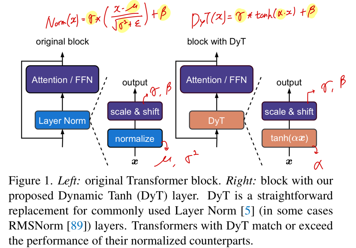
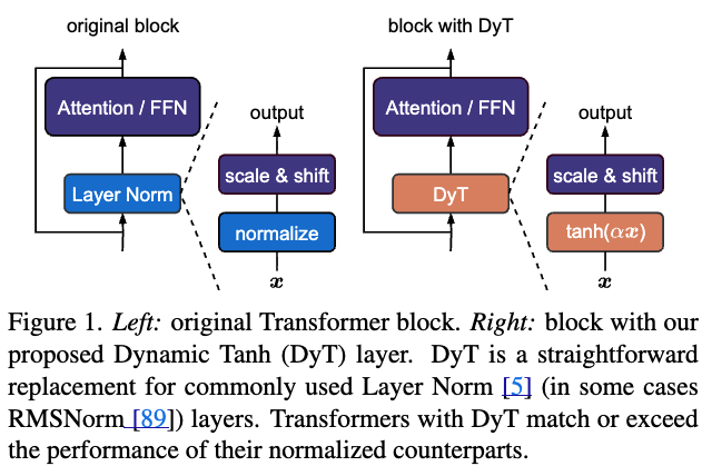
DyT를 적용하는 것은 Figure 1에 보이는 것처럼 간단하다:
vision and language Transformers와 같은 architectures에서 existing normLayers를 DyT로 바로 교체하면 된다.
우리는 경험적으로 models with DyT가 다양한 settings에서 can train stably and achieve high final performance임을 증명했다.
models with DyT는 보통 original architecture의 hyper-parameters tuning을 필요로 하지 않는다.
우리의 연구는 normLayer가 modern neural networks 학습에 필수적이라는 관념(notion)에 도전하며, normLayer의 properties에 대한 empirical insights를 제공한다.
2. Background: Normalization Layers
-
normLayer를 review하면서 시작한다.
Most normalization layers는 a common formulation을 공유한다.
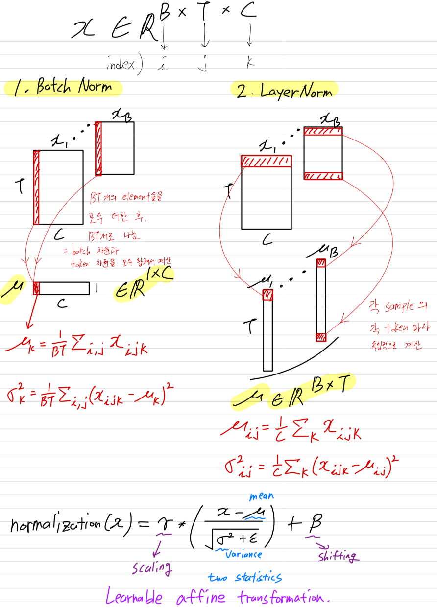
Give an input with shape , where is the batch size, is the number of tokens, and is the embedding dimension per token,
the output is generally computed as:
.
여기서 은 a small constant, and ("scaling") and ("shifting")는 learnable vector parameters of shape 이다.
와 는 input의 mean and variance를 나타낸다.
다른 methods들은 주로 이 두 개의 statistics를 계산하는가에 따라 달라진다.- 주로 ConvNets에서 사용되는 Batch Normalization (BN)에서는
and 로,
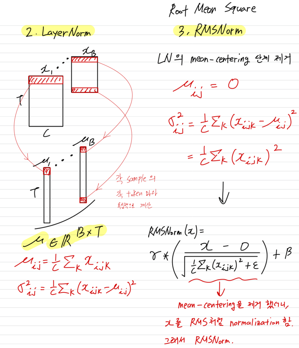
batch 차원과 token 차원을 모두 합쳐서 mean and variance를 계산한다. - 주로 Transformer architectures에서 사용되는 Layer Normalization (LN)에서는
and 로,
각 sample의 각 token마다 statistics를 독립적으로 계산한다. - 주로 Transformer architectures에서 사용되는 RMSNorm은 LN을 단순화한 것으로, the mean-centering 단계를 제거하고, input을 다음과 같이 normalizing한다.
and
- 주로 ConvNets에서 사용되는 Batch Normalization (BN)에서는
-
most modern neural networks에서는 LN의 simplicity and universality 덕분에 LN을 사용하고 있다.
최근에는 특히 language model에서 RMSNorm의 인기도 많아지고 있다. (T5, LLaMA, Mistral, Qwen, InternLM, DeepSeek)
이 논문에서 우리가 평가한 Transformers들은 LLaMA가 RMSNorm을 사용한 것을 제외하고, 모두 LN을 사용한다.
BN vs. LN vs. RMSNorm
요약)
input activation에 대해서 two statistics(mean=와 variance=)를 구하는 방법에 따라
BatchNormalization, LayerNormalization, RMSNorm으로 구분된다.
이 논문에서는 LLaMa 빼고, 모두 LN에 대해서 실험을 적용했다.
(질문) : Transformer에서 특히 RMSNorm이 많이 사용되고 있다고 했는데, 왜 Transformer에서만 특히 많이 사용될까?
(AI 답): Transformer는 residual connection이 많아서, mean-centering이 크게 중요하지 않다. 그래서 mean-centering을 빼도 충분히 안정적으로 학습될 뿐더러 더 단순하고 빠르다.
3. What Do Normalization Layers Do?
Analysis setup.
-
우리는 먼저 이미 trained된 networks에서 normalization layers의 behaviors를 경험적으로 연구했다.
이 분석을 위해,
(1) ViT-B trained on ImageNet-1K,
(2) a wav2vec 2.0 Large Transformer model trained on LibriSpeech,
(3) Diffusion Transformer (DiT-XL) trained on ImageNet-1K
를 가지고 실험했다.
모든 경우에서, LN은 모든 Transformer block에의 the final linear projection 이전에 적용되었다. -
위 세 가지 networks에 대해서, 우리는 mini-batch of samples을 샘플링하여 network에 forward pass를 진행했다.
그 다음 normalization layers의 input과 output을 측정했는데, 이는 normalization operation 직전과 직후 (learnable affine transformation = scaling()과 shifting())의 tensor를 의미한다.
LN은 input tensor의 dimension을 그대로 유지하므로, input과 output elements 사이에 one-to-one 대응 관계를 만들 수 있으며,
이를 통해 두 값의 relationship을 Figure 2에 나타냈다.

Tanh-like mappings with layer normalization.
-
세가지 model 전부에 대해,
earlier LN layers (1st column of Figure 2)에서 input-output relationship이 linear하며, x-y plot에서 straight line에 가까운 모습을 보임을 발견했다.
하지만 deepr LN layers에서 관찰한 놀라운 점은, tanh function으로 표현되는 완전하거나 부분적인 S-shaped curves를 띤다는 것이다. -
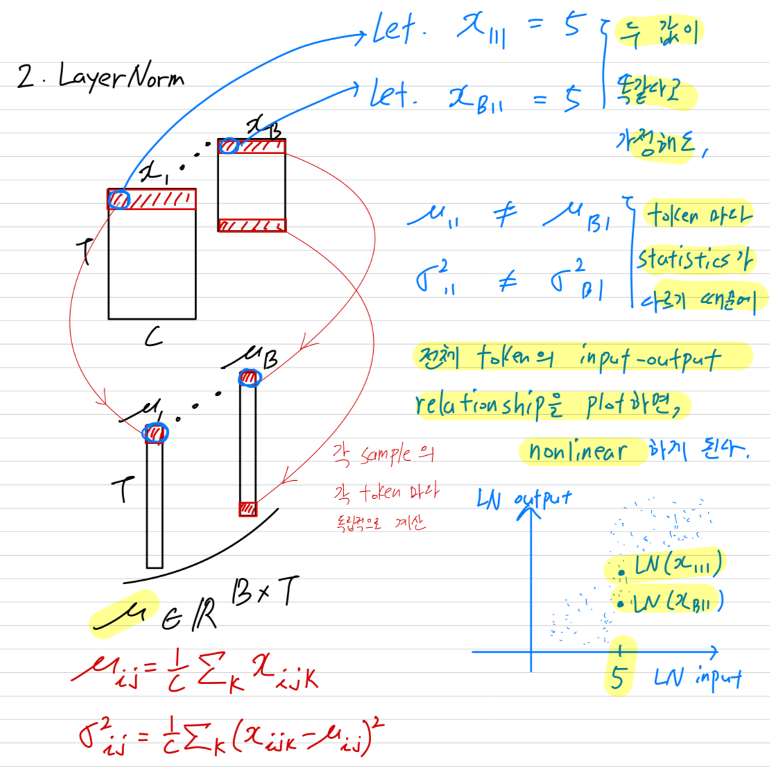
LN은 per-token 단위로 mean을 subtracting하고 standard deviation으로 dividing하기 때문에 input tensor를 linearly transform한다고 생각할 수 있지만...
token마다 mean and stddev 값이 다르기 때문에 모든 activation들을 하나로 모아서 보면 전체적으로는 linearity가 유지되지 않는다.
(정리: 즉, 개별 token 단위에서는 linear하지만 모든 activation값들을 모아서 그려보면 linearity가 깨진다. nonlinear하다.)
(AI의 쉬운 설명: 각 token은 직선 경로를 가지만, 모두 다른 속도(분산)과 방향(평균)으로 움직여서, 전체 무리를 보면 곡선을처럼 보이는 것과 같다.)
(아래 그림은 내가 이해한 내용)
-
모든 activation들을 하나로 모아서 그렸을 때, linearity가 깨지는 것은 알겠는데...
이러한 non-linear transformation이 scaled tanh function과 매우 유사하다는 것이 놀라운 것이다. -
S-shaped curve를 보면, 값이 0에 가까운 central part에서는 대부분 linear shape 구간에 놓여있다.
대부분의 points (약 99%)가 이 linear range에 존재한다.
하지만 이 range를 명확히 벗어나는 point들이 상당히 존재하는데, 이들은 "extreme" values로 간주된다.
예를 들어, ViT model에서는 값이 50보다 크거나 -50보다 작은 값들인 이에 해당한다.
normalization layer들이 이러한 extreme values에 주는 효과는 그 값을 less extreme values로 squash(밀어 넣다)한다는 것이다.
그렇기 때문에, normalization layer는 a simple affine transformation layer로는 approximation될 수 없다는 것이다.
우리는 extreme values에 대해 이렇게 non-linear하고 disprotional(불균형)한 squahsing effect가
normalization layers가 중요한 이유이자 필수적인 요소라는 가설을 세운다.
추가로, 최근에 Ni et al. [62]에서도 유사하게 LN layers의 strong non-linearities를 강조하며, non-linearity가 얼마나 a model's representational capacity를 강화하는지 보였다.
게다가 이러한 squashing behavior는 100년 전 쯤 관찰된 현상인, the saturation properties of biological neurons for large inputs을 모방한다.
(정리: LayerNormalization은 non-linearity의 특성을 가지고 있고, extreme value를 squash해주는 역할도 있기 때문에, a simple linear transformation으로 approximation할 수 없다.
즉, LayerNorm을 approximation하려면 non-linear transformation을 사용해야 한다.
저자들이 제안하는 non-linear 함수인 tanh()를 사용한 이유에 대해서 정당성을 부여하는 중요한 주장이었다고 생각함.)
Normalization by tokens and channels.
-
LN layer는 각 token에 대해서 a linear transformation을 수행하면서, 동시에 extreme values를 어떻게 그렇게 non-linear 방식으로 squash할 수 있을까?
이를 이해하기 위해, 우리는 points들을 token별, channel별로 각각 묶어서 시각화했다.
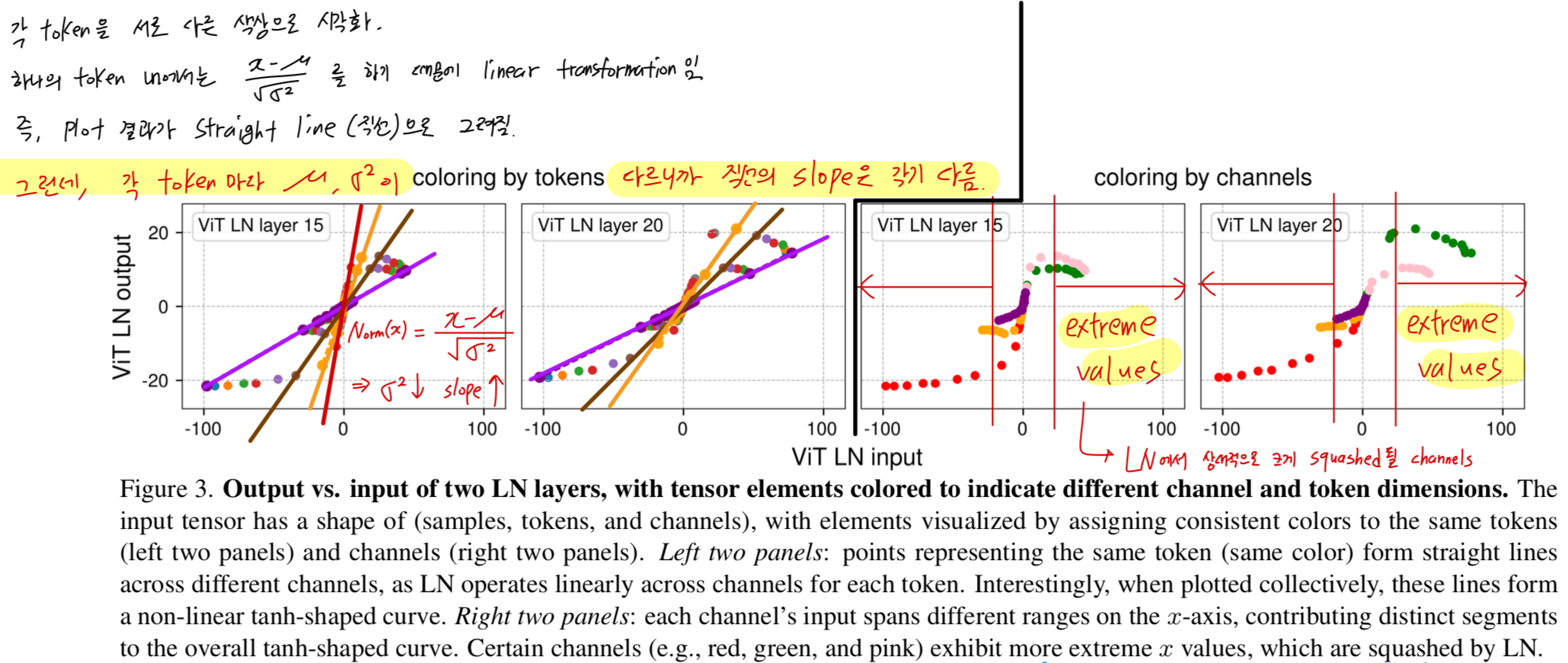
Figure 3에서는 Figure 2의 ViT 관련 두 번째, 세 번째 subplot을 가져와, 더 명확하게 보기 위해 sampling된 일부 점들만을 사용해 plot했다.
plotting할 channel을 선택할 때는 extreme values를 가지는 channel들을 반드시 포함하도록 했다. -
Figure 3 왼쪽 두 개의 panels에서, 우리는 각 token's activation을 동일한 색으로 표시했다.
관찰해보면, any single token에 속한 모든 points들은 straigh line(직선)을 이룬다.
( 하나의 token 내에서 mean, stddev를 구해 normalization하기 때문에 linear한 것이 당연)
하지만, token마다 variance가 다르기 때문에 각 직선의 기울기(slope)는 서로 다르다.
input 값의 범위가 작은 token일수록 variance가 작으며, normalization layer는 이 token의 activation을 더 작은 stddev로 나누게 된다.
그 결과, 기울기가 더 큰 직선이 형성된다.
이러한 직선들이 모두 합쳐지면, 전체적으로는 tanh()와 유사한 S-shaped curve를 이루게 된다.
(앞서 내가 그려놨던 그림과 동일한 내용이 Figure 3 left panel에서 말해주고 있었다...)
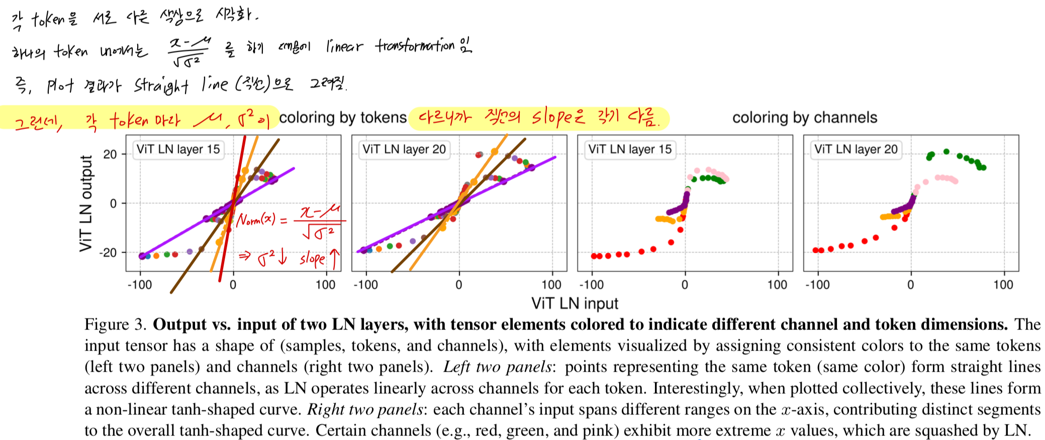
Figure 3 오른쪽 두 panels에서는, 각 channel의 activation을 동일한 색으로 표시했다.
여기서 우리는 channel별로 input value의 range가 매우 크게 다르다는 것을 확인할 수 있다.
특히 소수의 channel(예: red, green, pink)이 매우 큰 extreme values를 가진다.
이러한 channel들이 NormLayer에서 가장 크게 squashed되는 channel들이다.
4. Dynamic Tanh (DyT)
- normalization layers과 a scaled tanh function의 모양이 비슷한 것에서 영감을 받아, normalization layers를 대체하기 위한 Dynamic Tanh (DyT)를 제안한다.
input tensor 가 주어졌을 때, DyT layer는 다음과 같이 정의된다 :
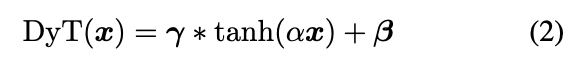 여기서, 는 입력의 range에 따라 서로 다른 방식으로 scaling할 수 있도록 해주는 a learnable scalar parameter로,
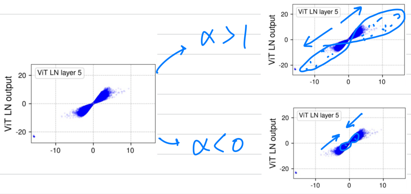
input 의 scale 변화(Figure 2에서 초기 layer는 tanh의 중심부처럼 linear한 형태를 갖고 후기 layer는 S-shaped curve를 갖는)를 보정한다.
이것이 우리가 whole operation을 "Dynamic" Tanh 이라고 부르는 이유이다.
(내가 이해한 내용: 아래처럼 input 의 scale 변화를 dynamic하게 만들 수 있도록 learnable parameter 를 학습.
Figure 2에서는 초기 Layer일수록 x-LN(x)의 relationship이 linear하고, 후기 layer일수록 x-LN(x)의 relation ship이 tanh shape을 갖는다는 특징들을 를 통해 학습할 수 있다는 것)
and 는 모든 normalization layers에서 사용되는 것과 동일한 방식 learnable, per-channel vector parameters이며,
이를 통해 output값을 다양한 scale로 되돌릴(back) 수 있다.
이는 종종 별도의 affine layer로 취급되지만, normalization layers가 affine transformation을 포함하듯이, 본 논문에서는 이들을 DyT layer의 일부로 간주한다.
PyTorch-like pseudocode of DyT는 Algorithm 1에 제시되어 있다.
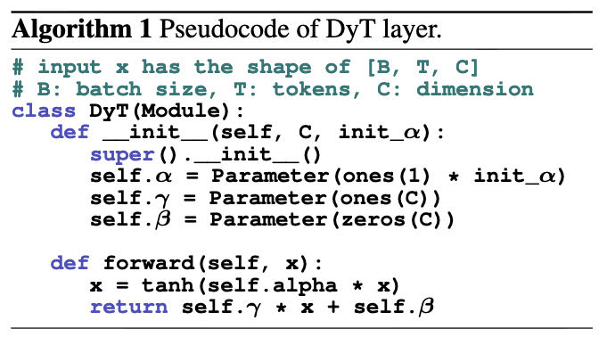
- DyT를 existing architecture에 통합하는 것은 매우 간단하다:
one DyT layer가 one normalization layer를 대체하면 된다 (Figure 1)
이는 attention block, FFN block, final normalization layer 내의 normalization layer에도 적용된다.
비록 DyT가 activation function처럼 보이거나 간주될 수 있지만, 이 연구에서는 GELU와 ReLU 같은 original architecture의 actiation function을 변경하지 않고 normalization layer만 대체하는 용도로 DyT를 사용했다.
network의 다른 부분들은 그대로 유지된다.
또한 DyT가 잘 동작하기 위해 original architectures의 hyperparameter를 크게 tuning할 필요가 없다는 것도 관찰했다.
On scaling parameters
-
scaling parameters에 대해서는, normalization layers에 따라
는 an all-one vector로 initialize하고
는 an all-zero vector로 initialize했다. -
scaler parameter 에 대해서는, LLM training을 제외하고, a default initialization of 0.5를 사용하는 것으로 충분했다.
별도로 명시되지 않는 한, 이후 experiments에서 는 0.5로 initialization되었다.
Remarks
- DyT는 a new type of normalization layer가 아니다.
DyT는 forward pass 동안 tensor의 각 input element에 대해 독립적으로 동작하며 statistics or other types of aggregation을 계산하지 않는다.
그러나 DyT는 input의 central parts를 거의 linearly tranforming하면서,
extreme values는 non-liner fashion으로 squashing하는 normalization layer의 효과를 그대로 유지한다.
주목할 점: DyT는 새로운 종류의 정규화 레이어는 아닙니다. DyT는 순전파(forward pass) 동안 텐서의 각 입력 요소에 대해 독립적으로 동작하며 통계나 기타 집계 연산을 계산하지 않습니다. 그러나 DyT는 입력의 중심 부분을 거의 선형으로 변환하면서, 극단적인 값들은 비선형 방식으로 압축(squash)하는 정규화 레이어의 효과를 그대로 유지합니다.
5. Experiments
- DyT의 effectiveness를 증명하기 위해, Transformers and a few other modern architectures across a diverse range of tasks and domains에 실험했다.
각 실험에서, 우리는 LN or RMSNorm in the original architectures를 DyT layers로 대체했다.
중요한 것은, adapting DyT의 simplicity를 강조하기 위해, 우리는 the normalized counterparst에 사용되었던 hyperparameters를 그대로 동일하게 사용했다.
Supervised learning in vision
- ViT and ConvNeXt of Base and Large sizes를 ImageNet-1K classification task에 train시켰다.
이 model들을 선택한 이유는 그들의 popularity and distinct operations 때문이다: attention in ViT and convolution in ConvNeXt.
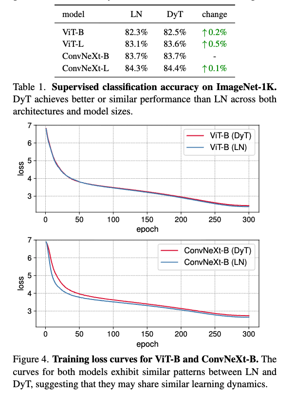
Table 1에 Top-1 classification accuracies를 보고했다.
DyT는 두 architectures and model sizes에서 LN보다 살짝 더 좋은 성능을 보였다.
추가로 Figure 4에서는 ViT-B, ConvNeXt-B에 대한 training loss를 plot했다.
training loss curves는 DyT와 LN-based model의 convergence behaviors가 align됨을 보여준다.
Self-supervised learning in vision
-
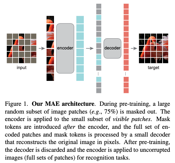
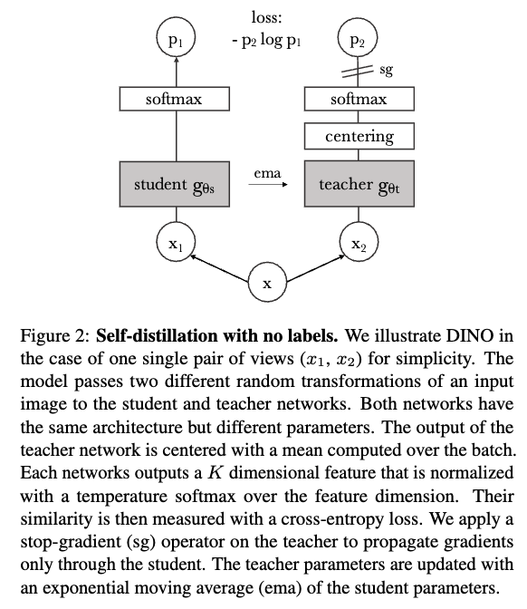
우리는 two popular visual self-supervised learning methods: masked autoencoders (MAE) and DINO를 benchmarking했다.
두 방법 모두 기본적으로 ViT를 backbone으로 사용하지만, training objectives가 다르다:
MAE는 reconstruction loss로 trained되고,
DINO는 joint-embedding loss로 trained 된다. -
the standard self-supervised learning protocol에 따라,
우리는 ImageNet-1K dataset에서 label 없이 pretrain하고,
그 후 pretrained model에 classification layer를 붙여 label을 사용해 fine-tuning 했다.
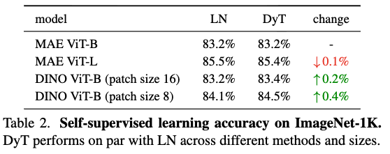
finetuning results는 Table 2에 나와있다.
결과적으로, DyT는 self-supervised learning tasks에서 LN과 동등한 성능을 지속적으로 보여준다.
참고
-
Masked Autoencoders ViT는 label이 없는 대규모 data를 사용하여 image의 강력한 feature representation을 효율적으로 학습하는 self-supervised learning 모델.
이 pretrained된 encoder는 이후 object detection, segmentation 등 다양한 downstream 작업의 backbone으로 사용.
(2021 CVPR, https://arxiv.org/pdf/2111.06377) -
작동 방식:
input image의 약 75%에 달하는 Patch를 random masking.
나머지 25%의 visible patch만 처리.
encoder는 극도로 작은 input만으로도 Image의 전체 context를 유추하도록 학습되어, 강력한 일반화 능력을 학습.
decoder는 encoder의 output(visible patch의 feature vector)와, masked된 위치를 채우는 Mask Tokens을 입력으로 받음.
decoder는 이 정보를 바탕으로 masked patch의 실제 pixel 값을 reconstruct하는 것.
-
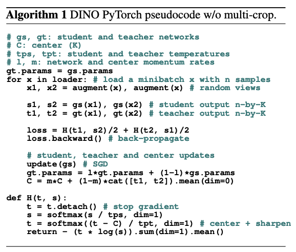
DINO ViT:
DINO는 DIstillation with NO labels의 약자로, 레이블 없이 지식 증류(knowledge distillation)를 사용하는 방식
(2021 ICCV, https://arxiv.org/pdf/2104.14294)
Diffusion models
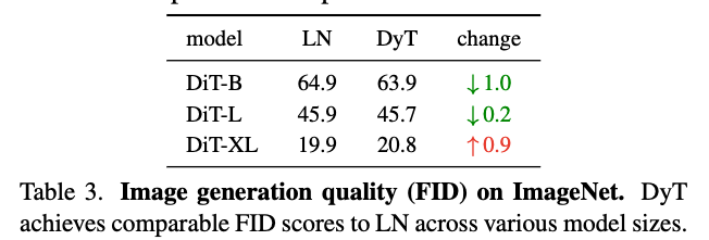
- 우리는 three Diffusion Transformer (DiT) models of sizes B, L and XL을 ImageNet-1K에 train했다.
patch size는 각각 4, 4, and 2이다.
DiT에서는 LN layer의 affine parameter가 class conditioning에 사용되므로, DyT 실험에서도 이 부분은 그대로 유지하고,
오직 normalizaing transformation만 로 대체했다.
training 후, standard ImageNet "reference batch"를 사용하여 Fréchet Inception Distance (FID) scores를 평가했으며, 결과는 Table 3에 제시되어 있다.
DyT는 LN과 비교했을 때 동등하거나 더 나은 FID를 달성.
(참고: Fréchet Inception Distance (FID) scores 란? generative model이 만들어낸 image의 quality와 diversity를 평가하는 데 사용되는 지표, 실제 ground truth 분포와 생성된 image 분포 간의 통계적 유사성을 측정. 0에 가까울 수록 두 분포가 완벽하게 일치하는 이상적인 모델.)
Large Language Models
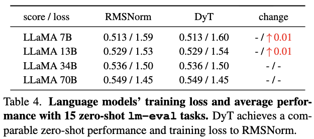
- 우리는 LLaMA 7B, 13B, 34B, 70B model을 pretrain하여 DyT가 LLaMA에서 기본적으로 사용되는 RMSNorm 대비 성능을 평가했다.
model은 The Pile dataset의 200B token으로 학습되었으며, LLaMA에서 제시한 original recipe을 따랐다.
DyT를 적용한 LLaMA에서는 initial embedding layer 뒤에 a learnable scalar parameter를 추가하고, 의 initial value를 조정했다. (자세한 내용은 Section 7)
학습 후 loss값을 보고했으며, OpenLLaMA를 따라 lm-eval의 15개 zero-shot task에서 model을 benchmarking했다.
Table 4에 나타난 것처럼, DyT는 네 가지 모델 크기 모두에서 RMSNorm과 동등한 성능을 보였다.
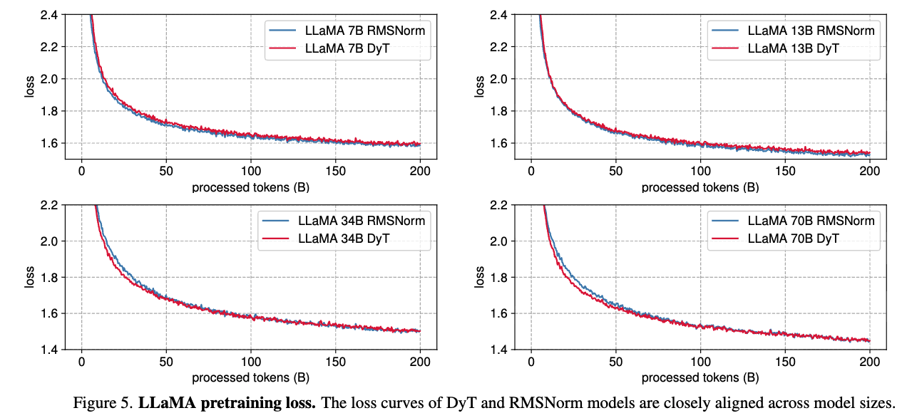
Figure 5는 loss curves를 보여주며, 모든 model sizes에서 유사한 경향을 나타내고 training loss가 training 내내 밀접하게 aligned됨을 확인할 수 있다.
6. Analysis
- 우리는 tanh function and the learnable scale 의 역할에 대해 실험을 진행했다.
6.1. Ablations of tanh and
- tanh and in DyT의 역할을 들여다보기 위해,
우리는 these components들이 교체되거나 제거되었을 때의 model's performance를 평가하는 실험을 수행했다.
Replacing and removing tanh.
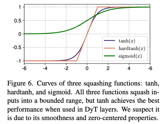
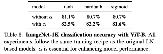
- DyT layer에서 tanh를 다른 squashing functions인 hardtanh와 sigmoid로 대체하고(Figure 6), learnable scalar 는 그대로 유지했다.
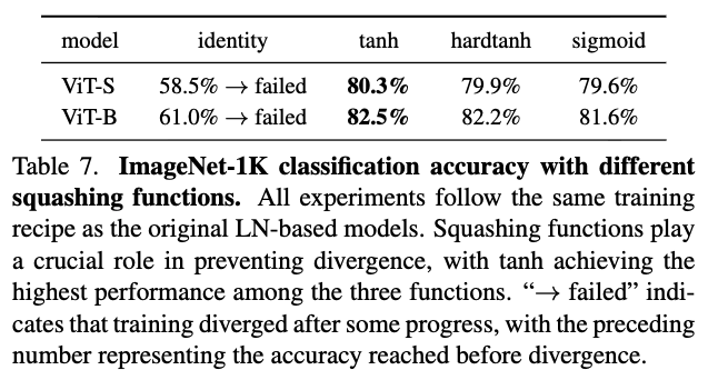
또한, tanh를 완전히 제거하고 identity로 바꾸되, 는 그대로 두었을 때의 영향을 평가했다.
Table 7에서 알 수 있듯이, squashing function은 squashing function은 stable training을 위해 필수적이다.
identity function을 사용하면 Unstable training and divergence를 유발하는 반면, squashing function을 사용하면 stable training이 가능하다.
squashing function 중에서는 tanh가 가장 좋은 성능을 보였는데, 이는 tanh가 smoothness and zero-centered properties를 가지기 때문일 가능성이 있다.
Removing
- 그 다음, 우리는 squashing functions을 유지한 채 learnable 를 제거하는 영향을 평가했다.
Table 8에 보이는 것처럼, removing 는 all squashing functions에서 performance degradation을 유발했고,
이는 the critical role of 를 강조한다.
6.2. Values of
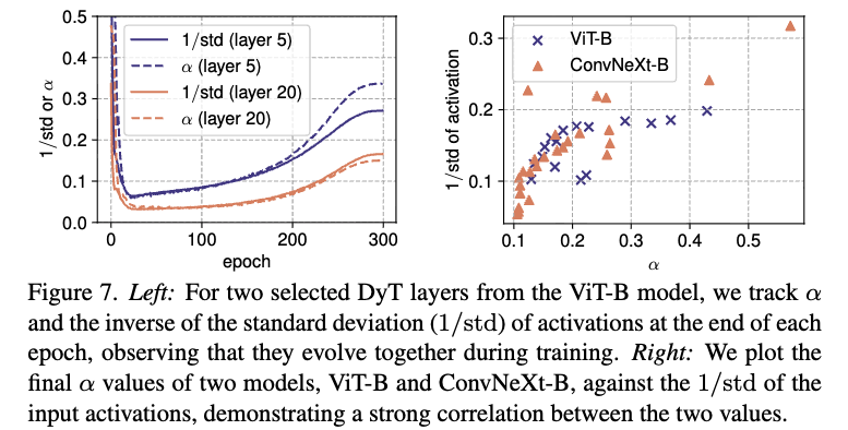
During training.
학습 중 analysis 결과, 는 training 내내 activation의 를 밀접하게 track하는 것으로 나타났다.
Figure 7의 left panel에서 볼 수 있듯, 는 학습 초기에 감소했다가 이후 증가하지만,
항상 activations의 standard deviation과 일관되게 변동한다.
이는 를 적절한 range 내로 유지하여 stable and effective learning을 가능하게 하는 important role임을 뒷받침한다.
(내 해석: 기존에 normalization layer에서 로 나누어 activation 값의 크기를 조정하는 역할을, 가 학습 동안 내내 유사한 scaling 효과를 학습하고 있다...)
After training.
학습 후 trained networks에서 의 final values를 분석한 결과, input activations의 과 강한 correlation을 보였다.
Figure 7의 right panel에서 볼 수 있듯, 값이 클수록 값도 크게 나타나고, 반대로 낮을수록 값도 작아진다.
또한, deeper layers일수록 activation 값의 standard deviations이 더 큰 경향이 있다.
이 경향은 [11] for ConvNet, [74] for Transformers에서 보여준 deep residual networks의 특성과 일치한다.
- 두 분석 모두 가 일종의 normalization mechanism 역할을 하며, input activation 값의 에 근접한 값을 학습함을 시사한다.
단, LN이 per token으로 normalize하는 것과 달리, 는 전체 input을 통합하여 normalize하며 extreme values를 non-linearly하게 억제할 수는 없다.
7. Initialization of
- 우리는 의 initialization(denoted )이 대부분의 경우 성능 향상에 큰 영향을 주지 않는다는 것을 발견했다.
유일한 예외는 LLM training으로, 이 경우 를 careful tuning하면 noticeable performance gains을 얻을 수 있다.
이 section에서는 initialization의 영향에 대해 자세히 설명한다.
7.1. Initialization of for Non-LLM Models
-
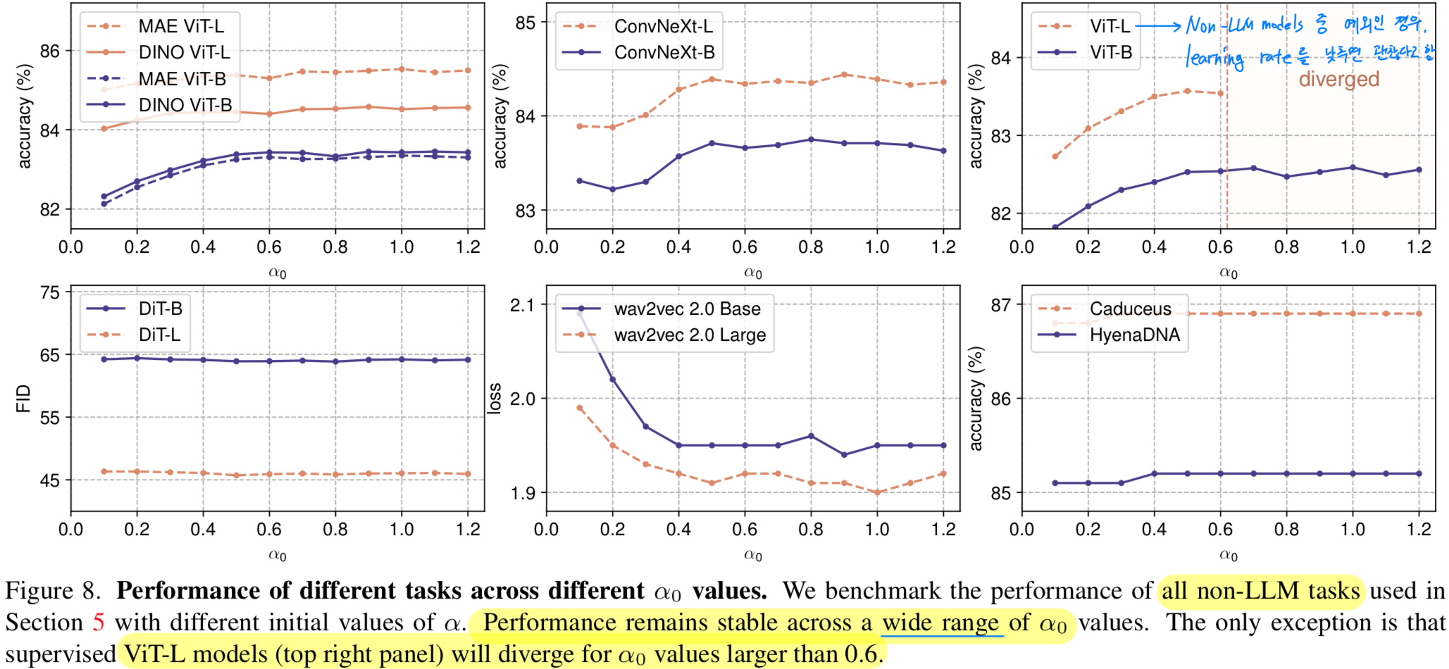
Non-LLM models은 에 상대적으로 insensitive하다.
Figure 8은 다양한 task에서 값을 변화시켰을 때 validation performance에 미치는 영향을 보여준다.
모든 실험은 각 model의 original setup and hyperparameters를 따른다.
우리는 값이 넓은 범위에 걸쳐도 성능이 안정적으로 유지되며, 일반적으로 0.5에서 1.2 사이의 값이 좋은 결과를 낸다는 것을 관찰했다.
를 조정하는 것은 일반적으로 the early stage of the training curves에만 영향을 미친다.
주요 예외는 supervised ViT-L experiment로, 가 0.6을 초과하면 tranining이 unstable해지고 diverge한다.
이런 경우, learning rate를 낮추면 stability가 회복된다.
-
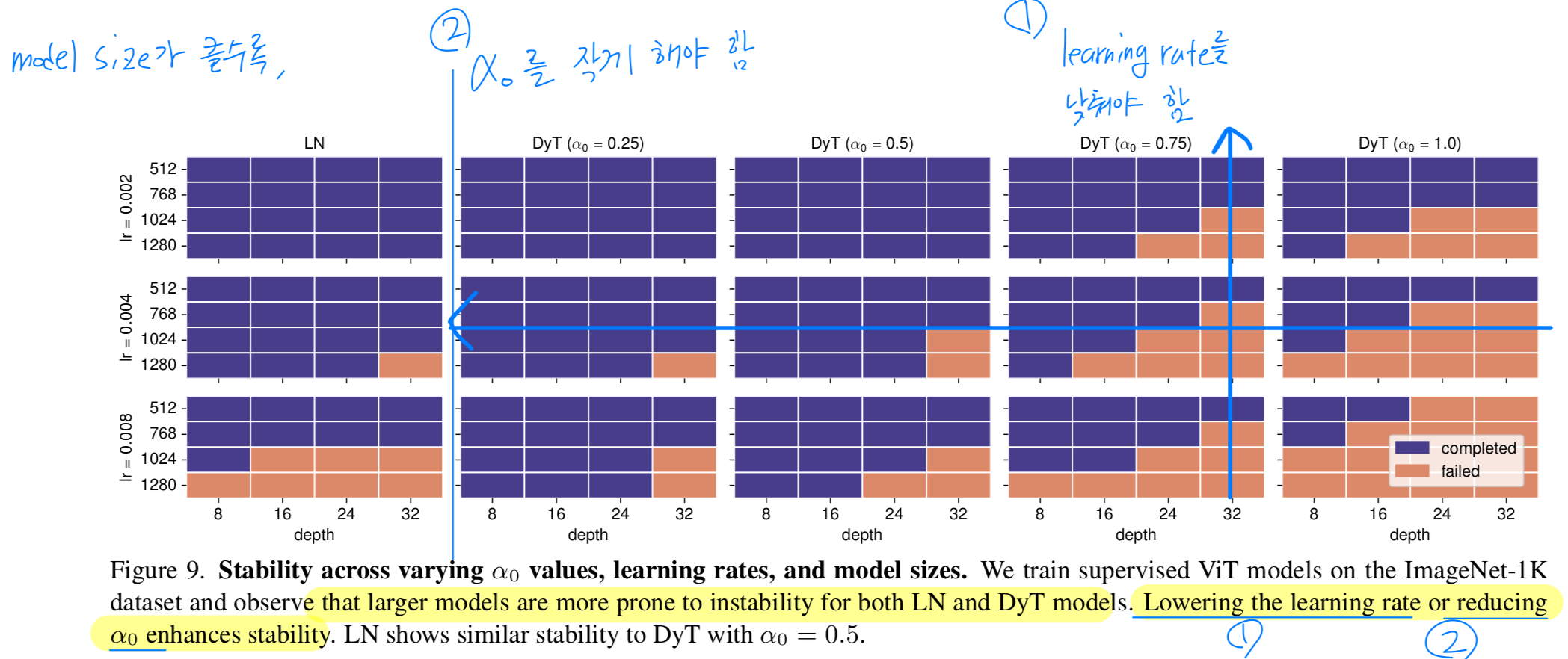
Smaller results in more stable training.
이전 observations을 바탕으로 training instability에 기여하는 요인을 추가 분석했다.
그 결과, model size or the learning rate를 증가하면 학습을 안정시키기 위해 를 낮춰야 한다는 것을 알 수 있다.
반대로 가 높으면 training instability를 줄이기 위해 lower learning rate가 필요하다.
Figure 9는 ImageNet-1K dataset에서 supervised learning ViT의 training stability에 대한 ablation을 보여준다.
learning rates, model sizes, and values를 변화시키며 실험했다.
큰 model을 학습할수록 failure 가능성이 높아지며, 안정적인 학습을 위해 smaller values or learning rates가 필요하다.
유사한 instability pattern이 LN-based models에서도 관찰되며, 로 설정하면 LN과 유사한 stability pattern을 보인다.
-
our findings를 기반으로, 우리는 all non-LLM models에 대해 default value를 로 설정했다.
7.2. Initialization of for LLMs
- Tuning enhances LLM performance.
앞에서 discussed했듯이, 대부분의 tasks에서 는 일반적으로 좋은 성능을 보인다.
그러나 를 tuning하면 LLM performance를 크게 향상시킬 수 있음이 확인되었다.
우리는 각 LLaMA model을 30B token으로 pretraining하고 training losses를 비교하여 를 tuning했다.
Table 9에는 각 model에 대한 tuned 값이 요약되어 있다.
Two key findings는 다음과 같다:- Larger models require smaller .
작은 model에서 optimal 를 찾으면, larger models의 search space그에 맞춰 줄일 수 있다. - Higher values for attention blocks improve performance.
attention block의 DyT layer에는 higher value로 initializing하고,
other locations(i.e., within FFN blocks or before the final linear projection)의 DyT layer에는 작은 values로 초기화하면 성능이 개선된다.
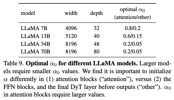
- Larger models require smaller .
8. Related Work
Normalization in Transformers
- Transformer의 등장과 함께, 연구는 점점 Layer Normalization에 주목하게 되었으며, 이는 특히 NLP tasks와 같은 sequential data에서 효과적인 것으로 입증되었다.
최근 연구에서는 LN이 strong non-linearity를 도입하여 model의 representational capacity를 향상시킨다는 사실을 보여줬다.
또한, 다른 연구들에서는 Transformers 내부에서 normalization layer의 위치를 조정하면 convergence properties를 개선할 수 있음이 확인되었다.
Removing normalization
-
많은 연구들은 deep models을 normalization layers 없이 학습시키는 방법을 탐구하고 있다.
몇몇 연구들은 training을 stabilizing하기 위해 alternative weight initialization 방식을 제안했다.
Self-normalizing networks는 scaled exponential linear units (SELUs)와
신중히 선태된 initialization 방식을 도입하여, 명시적인 normalization layer 없이도 stable activations and gradient flow를 유지했다.
[11, 12]의 연구에서는, ResNet을 높은 성능으로 학습할 수 있음을 보여줬는데, 이는 initialization techniques, weight normalization 그리고 adaptive gradient glipping이 포함된다.
위 연구들은 주로 다양한 ConvNet models을 기반으로 한다. -
Transformer architectures에는, [32]에서 normalization layer와 skip connections에 대한 reliance를 줄이는 Transformer block 의 modification을 탐구했다.
[42]는 AERO, 즉 Softmax만 사용하는 LLM을 소개하며, 성능 저하를 최소화하면서 inference efficiency and privacy를 개선했다.
[35]는 pretrained network에서에서 LN을 점진적으로 제거하고 각 normLayer를 제거한 후 model을 fine-tuning하는 방법을 제안했다.
이전 접근법과 달리, DyT는 architecture와 training recipe에 대한 수정이 최소화되어 있다.
DyT의 simplicity에도 불구하고, DyT는 stable training and comparable performance를 달성한다.
9. Limitations
- 우리는 LN 또는 RMSNorm을 사용하는 Network에서 실험을 수행했다.
이는 Transformers와 다른 modern architectures에서 두 normLayer 기법이 널리 사용되기 때문이다.
Appendix E에서는 DyT가 ResNet과 같은 classic networks에서 BN을 직접 대체하는 데 어려움이 있음을 보인다.
DyT가 다른 유형의 normalization layers를 사용하는 model에 어떻게 adapt할 수 있는지에 대해서는 추가적인 심층 연구가 필요하다.
Discussion
- normalization layer를 없애는 것이 어떠한 장점이 있길래...? 관련 연구도 그렇고, 왜 normalization layer를 없애려는 시도가 있는 것인가?
- normalization layer를 DyT로 대체함으로써 뻗어나갈 수 있는 연구, 응용이 분명 많을 거 같은데...
예를 들어, slimmable neural network에서 서로 다른 width configuration에 대응하도록 switchalbe BN을 학습시켰는데,
이 switchable BN (즉, 다른 network 구성에 따른 statistics 학습 과정)이 필요 없게 될 수도 있을까?
일단, 이 연구에서는 LN, RMSNorm을 target NormLayer로 했고 limitations에서 BN에서는 적용이 잘 안되었다고 명확히 언급했다.
이에 대한 추가 분석과 연구가 필요해 보임.
- normalization layer를 DyT로 대체함으로써 뻗어나갈 수 있는 연구, 응용이 분명 많을 거 같은데...
Seminar 발표 자료 공유
https://github.com/HyungseopLee/Paper_Review/blob/main/Paper-Review/251202_DyTanh.pptx
