Week 4 | Deep Neural Networks | Deep Neural Network
Deep L-layer Neural Network
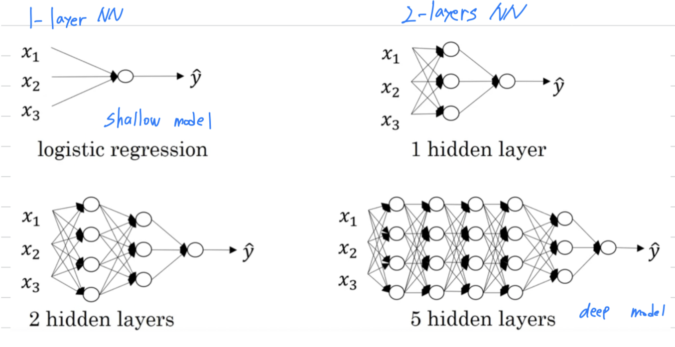
- We say that
logistic regressionis a very "shallow" model. - Whereas
5 hidden layersis a much "deeper" model. - technically logistic regression is a 1-layer neural network.
But over the last several years the AI on the machine learning community
has realized that there are functions that very deep neural networks can learn that shallower models are often unable to.
Deep neural network notation
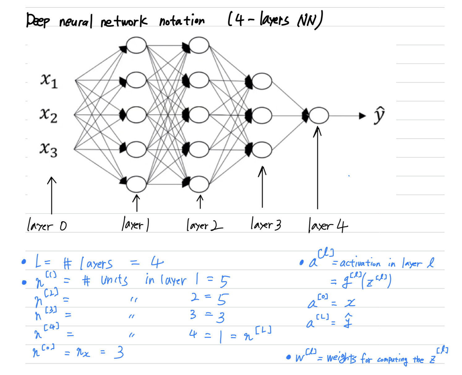
- : the number of layers in the network.
- : the number of nodes, or the number of units in layer .
- : the activation in layer .
- : the weights for computing the value . ()
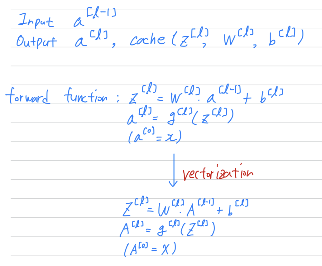
Forward Propagation in a Deep Network
single training example
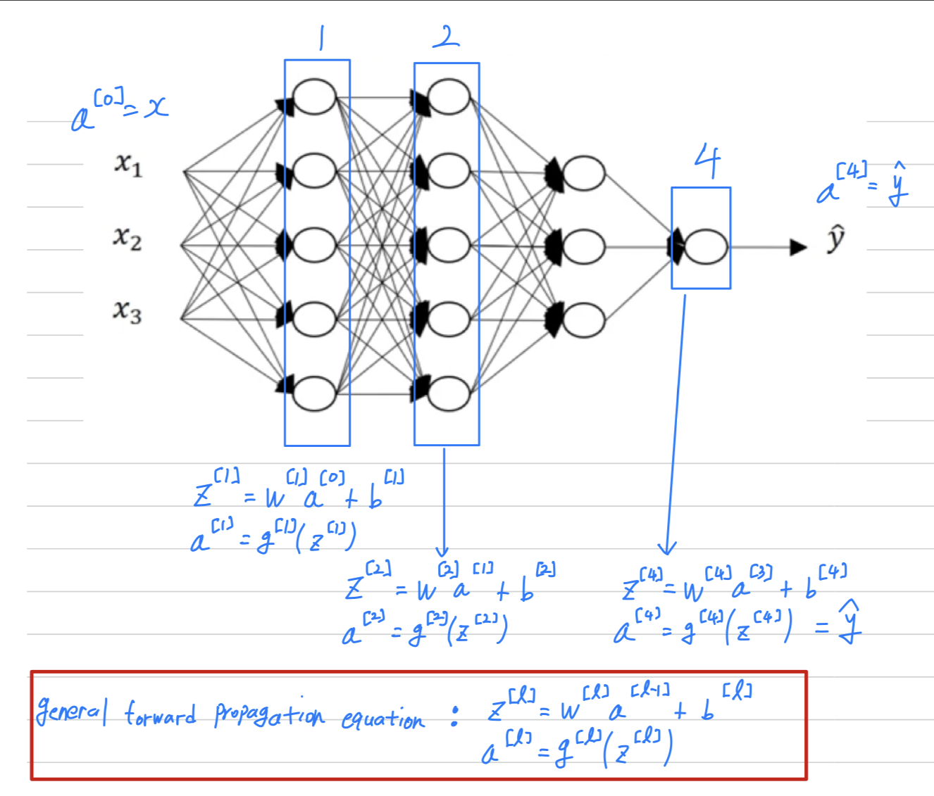
vertorized version
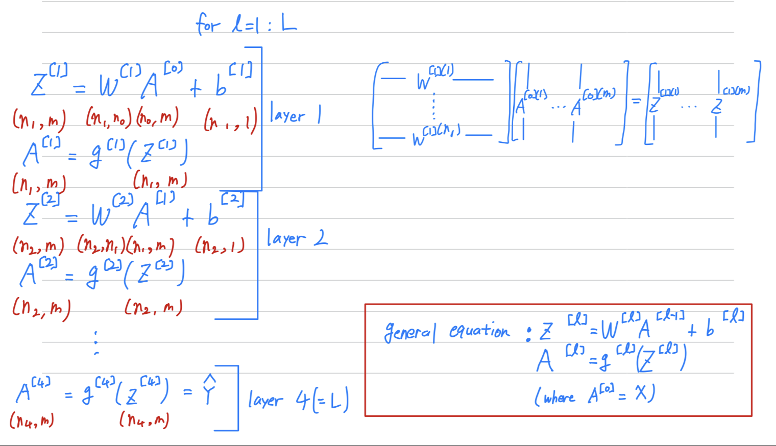
One of the ways to increase your odds of having a bug-free implementation is to think very systematic and carefully about the matrix dimension's you're working with.
Getting your matrix dimension right
- When implementing a deep neural network,
one of the debugging tools Ng often uses to check the correctness of his code
is to pull a piece of paper and just work through the dimensions in matrix he's working with.
single training example
- Of course, if you're implementing back-propagation,
then the dimensions of should be the same as dimension of .
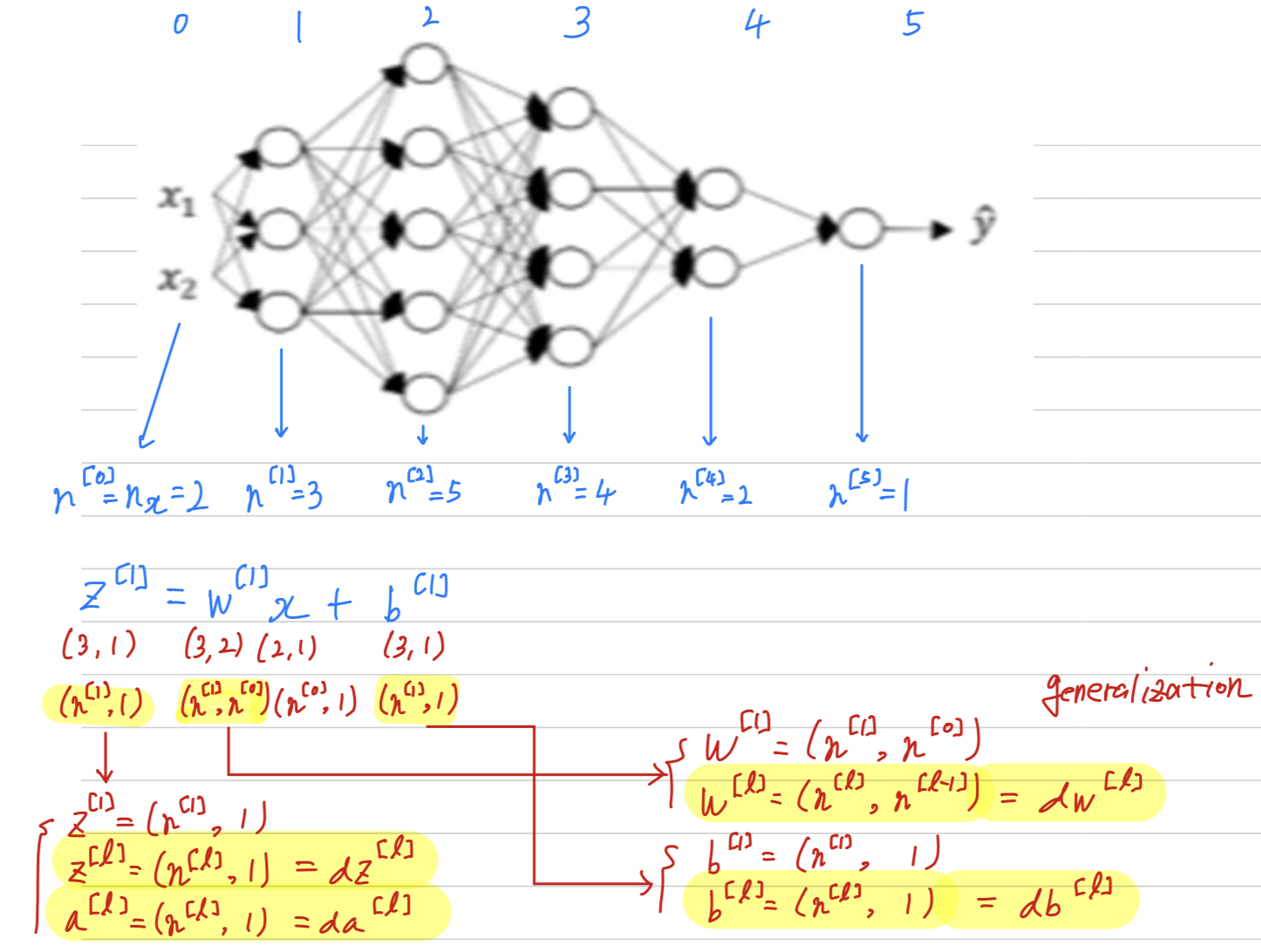
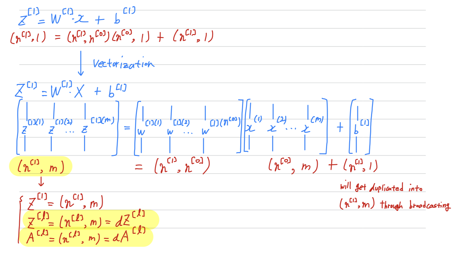
vectorized implementation
- Even for a vectorized implementation, of course,
, and will stay the same. - But the dimensions of will change a bit.
Why deep representations?
- Why are deep neural networks so effective and
Why do they do better than shallow representations?
Intuition about deep representation
-
So first,
what is a deep network computing? -
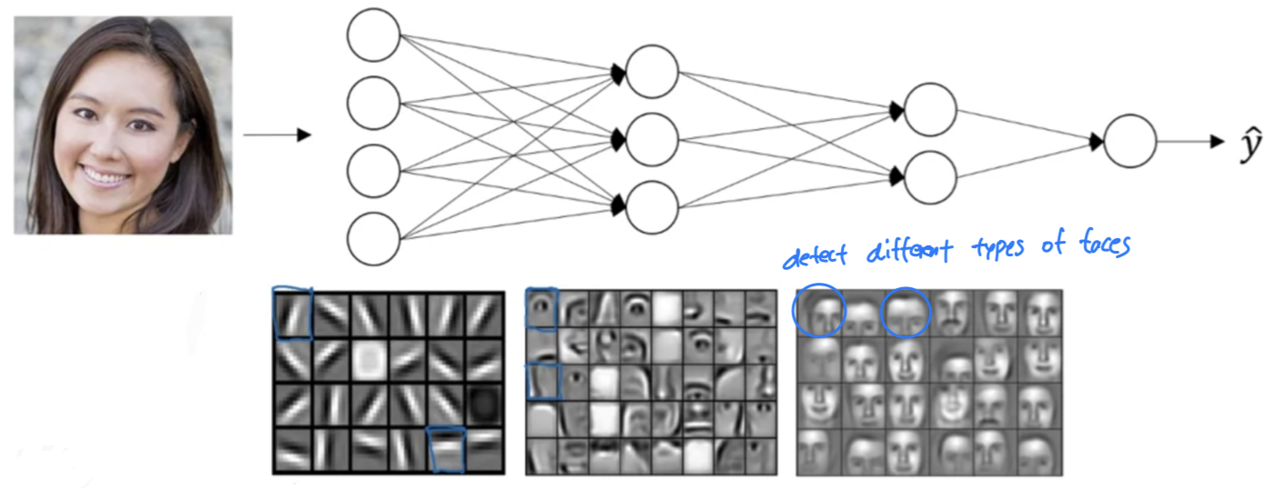
If you're building a system for face recognition,
here's what a deep neural network could be doing. -
Perhaps you input a picture of a face
Then the first layer of the neural network
you can think of as maybe being a feature detector or an edge detector.- In this example, i'm plotting what a neural network with maybe 20 hidden units,
might be trying to compute on this image.
So the 20 hidden units visualized by these little square boxes.
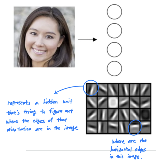
- In this example, i'm plotting what a neural network with maybe 20 hidden units,
-
Now, let's think about where the edges in this picture by grouping together pixels to form edges.
It can then detect the edges and group edges together to from parts of faces.- For example, you might have a low neuron trying to see if it's finding an eye,
or a different neuron trying to find that part of the nose.
And so by putting together lots of edges,
it can start to detect different parts of faces.
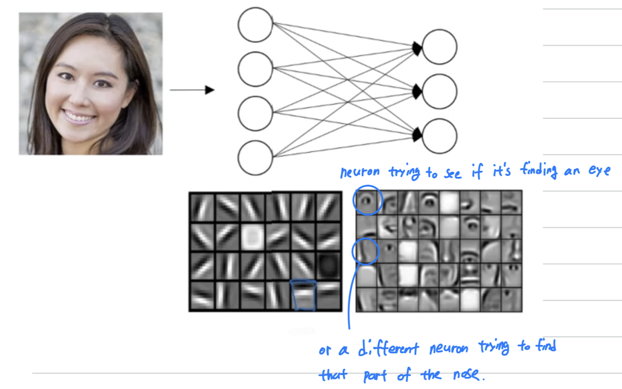
- For example, you might have a low neuron trying to see if it's finding an eye,
-
And then, finally, by putting together different parts of faces like an eye or a nose or an ear or a chin,
it cat then try to recognize or detect different types of faces.
-
So intuitively, you can think of the earlier layers of the neural network
as detecting simple functions, like edges.
And then composing them together in the later layers of a neural network
so that it can learn more and more complex functions. -
it's hard to visualize speech but

- if you input an audio clip then maybe the first level of a neural network
might learn to detect low level audio waveform features,
such as is this tone going up? is it going down? is it white noise or sniffling sound? what is the pitch? - And then by composing low level wave forms, maybe you'll learn to detect basic units of sound (phonemes).
for example, in the word "CAT", the "C" is a. phoneme, the "A" is a phoneme, the "T" is another phoneme. - But learns to find maybe the basic units of sound and
then composing that together maybe learn to recognize words in the audio. - And then maybe compose those together,
in order to recognize entire phrases or sentences.
- if you input an audio clip then maybe the first level of a neural network
So deep neural network with multiple hidden layers
might be able to have the earlier layers learn these lower level simple features of the input such as where the edge is,
and then have the later deeper layers then put together the simpler things it's detected
in order to detect more complex things such as detect faces or detect words or phrases or sentences.
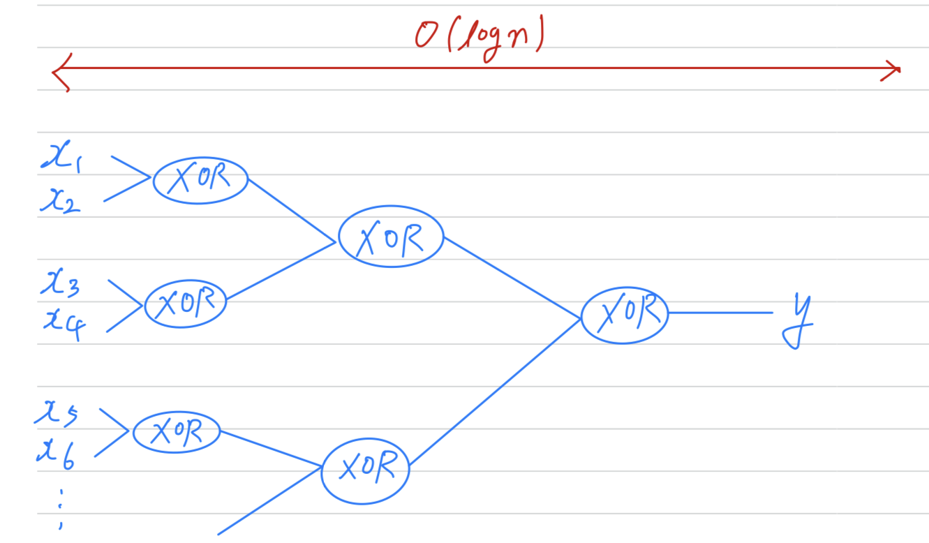
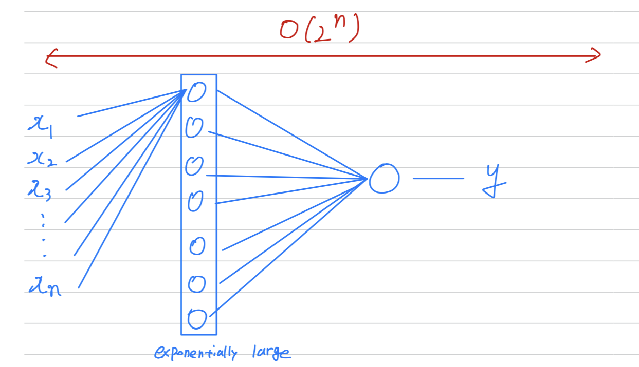
Circuit theory and deep learning
Informally : There are functions you can compute with a "small(the number of hidden units is small)" L-layer deep neural network.
But if you try to compute the same functino with a shallower network,
so if there aren't enough hidden layers,
then you might require exponentially more hidden units to compute.
-
Let's say you're trying to compute the exlusive OR.

-
But now,
if you are not allowed to use a neural network with multiple hidden layers with,
if you're forced to compute this function with just one hidden layer,
Then in order to compute this XOR function, hidden layer will need to be exponentially large, because essentially, you need to exhaustively enumerate our possible configurations.
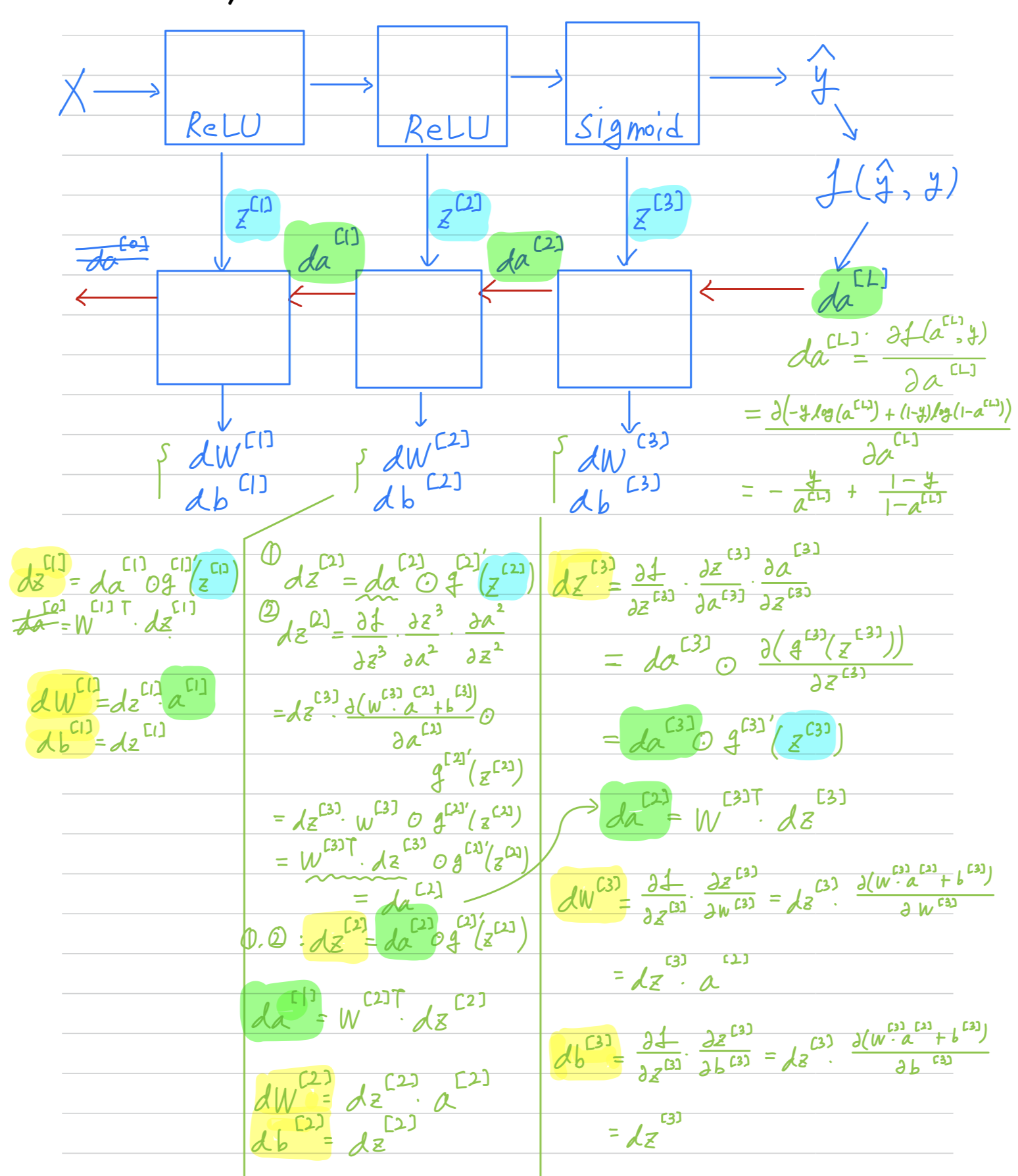
Building blocks of deep neural networks
-
We've already seen the basic building blocks of forward propagation and back propagation
, the key components you need to implement a deep neural network. -
Let's see how you can put these components to build our deep net.
Here's a network of a few layers.
Let's pick one layer.
And look into the computations focusing on just that layer for now.
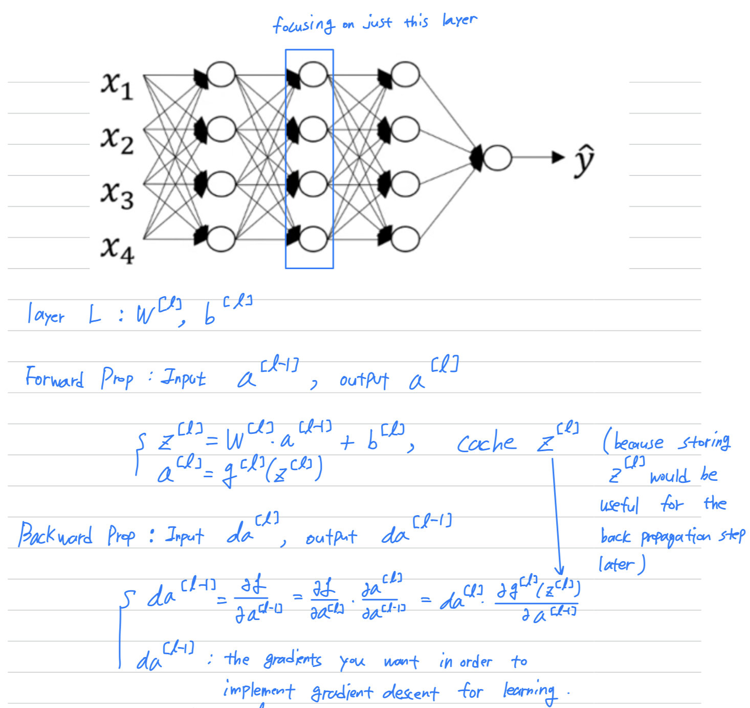 So just to summarize
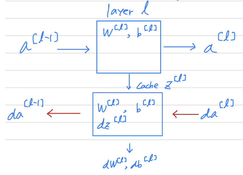
Forward and backward functions
-
So if you can implement these two functions
then the basic computation of the neural network will be as follows.
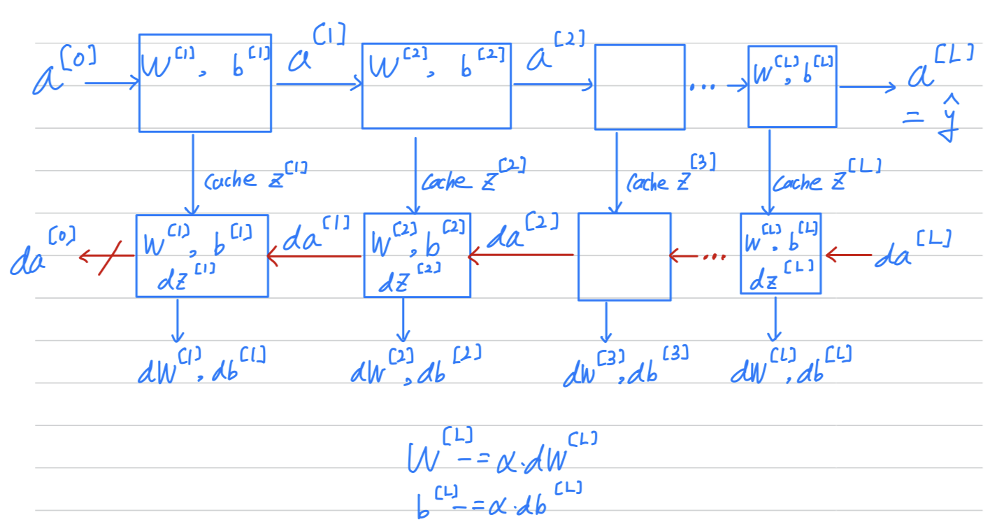 So one iteration of gradient descent for our neural network involves :
 - starting with which is and going through forward prop as follows.
- Computing and then using that to compute
- and then back prop, now you have all those derivative terms,
for each of the layers and similarly for () - would get updated
-
One more informational detail.
Conceptually, it will be useful to think of the cache
as storing the value of for the backward functions.
When you implement this,
you find that the cache may be a convenient way to get to this value of the parameters of into the backward function as well.
this exercise you actually store in your cache to as well as
Ng just finds it a convenient way to just get the parameters,
copy to where you need to use them later when you're computing back propagation.
(that's an implementational detail that we see when we do the programming exercise.)
Forward and Backward Propagation
Forward propagation for layer
Backward propagation for layer
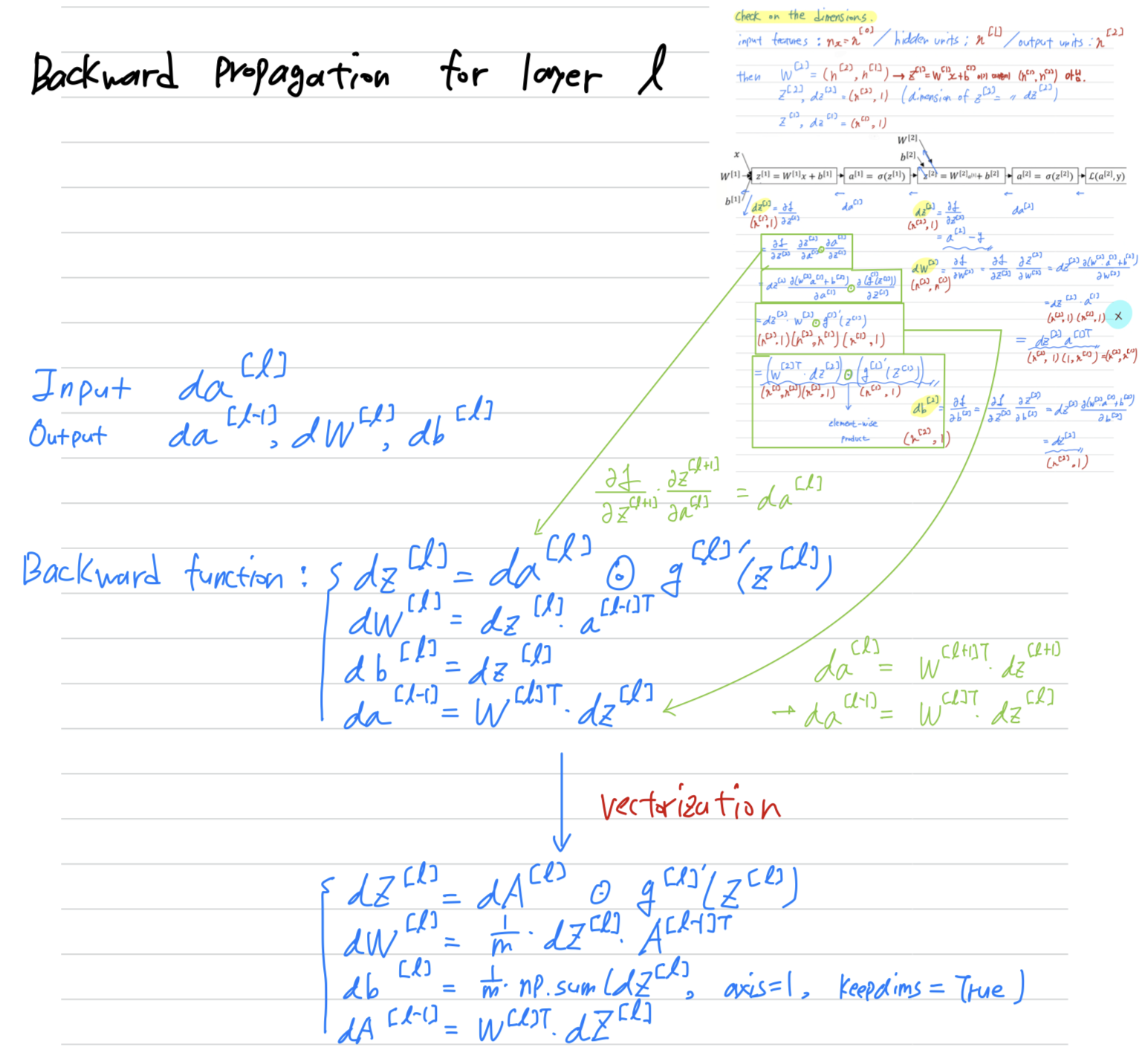
Summary
Parameters vs Hyperparameters
-
Parameters: and -
Hyperparameters- learning rate ()
- the number of iterations of gradient descent you carry out
- the number of hidden layers ()
- the number of hidden units ()
- choice of activation function (sigmoid, tanh, sigmoid, ...)
- later (momentum term, mini batch size, various forms of regularization parameters,...)
-
So when you're training a deep net for your own application you find that there may be a lot of possible settings for the hyperparameters that you need to just try out.
-
So applying deep learning today is a very empirical process where often you might have an idea.
It turns out that when you're starting on the new application, you should find it very difficult to know in advance exactly what is the best value of the hyperparameters.
So, what often happens is you just have to try out many different values and go around this cycle your try out some values, really try five hidden layers.
With this many number of hidden units implement that, see if it works,
and then iterate.
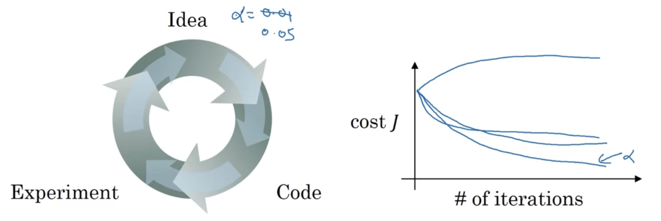
-
This is one area where deep learning research is still advancing.
(In the second course, we'll also give some suggestions for how to systematically explore the space of hyper parameters)
What does this have to do with the brain?
-
In this picture of a biological neuron,
this neuron, which is a cell in your brain,
receives electric signals from other neurons, or may from other neurons
does a simple thresholding computation
and then if this neuron fires,
it sends a pulse of electricity down the axon(축삭), perhaps to other neurons.
There is a very simplistic analogy between a single neuron in a neural network,
and a biological neuron.
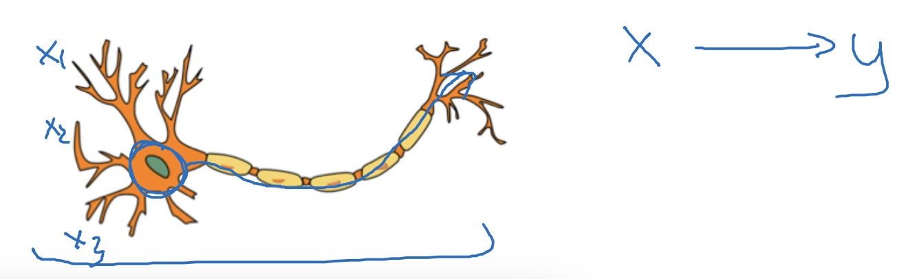
-
But Ng thinks that today even neuroscientists have almost no idea
what even a single neuron is doing.
A single neuron appears to be much more complex than we are able to characterize with neuroscience,
and while some of what it's doing is a little bit like logistic regression,
there's still a lot about what even a single neuron does that no one human today understands.
Semina - discussion
-
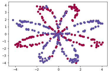
logistic regression의 accuracy가 왜 작은가?- 우선 원래의 planar data set을 plotting해보면, 다음과 같다.
의 2차원의 input feature와 에 해당하는 label이 있다.
or 이다.
즉, Binary-class classification problem이다.
- 만약 logistic regression을 사용한다면, Forward propagation은 다음과 같다.
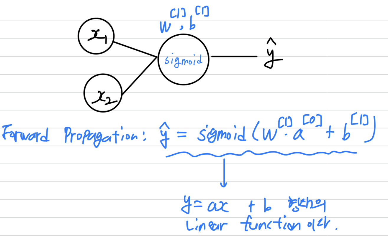
- 형태의 linear function이라는 의미는
2 dimension의 input feature 를 분류하기 위해 1차 linear function만이 사용된다는 의미이다.
따라서 2차원의 공간을 1차 linear function으로 아무리 classification해봤자, 두 영역으로만 나누어질 수 밖에 없다.
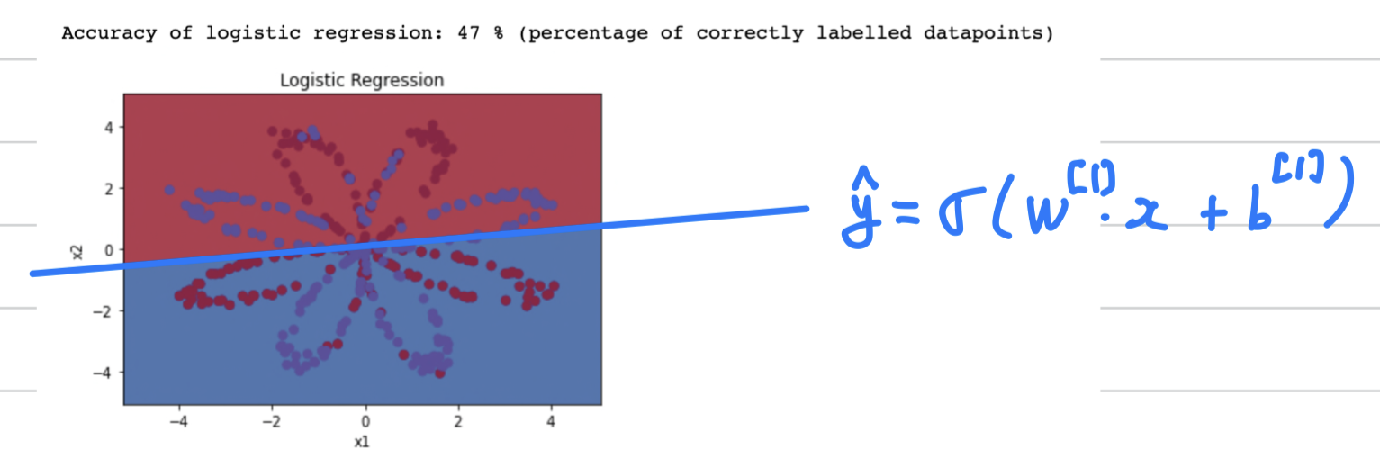
그러면 곡선으로 그어야 할 것이다.
라는 함수에
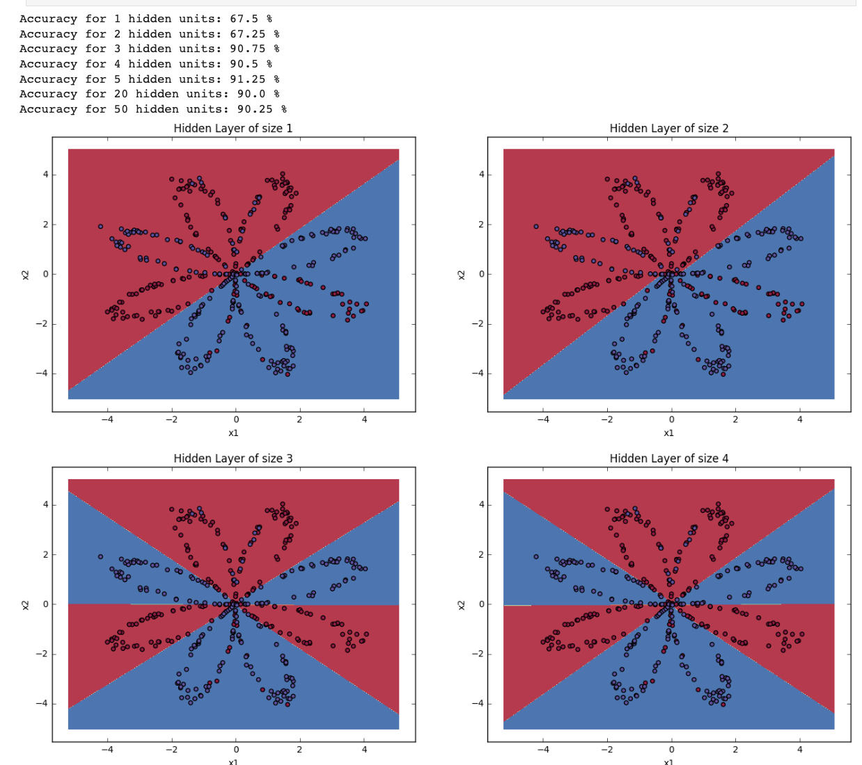
2 hidden layers 이상 + nonlinear activation function이면,
더욱 powerful한 NN이 될 수 있다.
== planar data를 더 잘 classification 할 수 있다.
- 우선 원래의 planar data set을 plotting해보면, 다음과 같다.
-
np.random.rand vs np.random.randn
- np.random.randn : randn generates an array of shape (d0, d1, ..., dn)
, filled with random floats sampled
from a univariate “normal” (Gaussian) distribution of mean 0 and variance - np.random.rand : Create an array of the given shape and populate it with random samples from a uniform distribution over [0, 1).
만약 weight initialization으로 np.random.rand() * 0.01을 사용한다면
0 ~ 0.01 사이의 값만 나오기 때문에 learning이 제대로 되지 않을 것이다.
- np.random.randn : randn generates an array of shape (d0, d1, ..., dn)
-
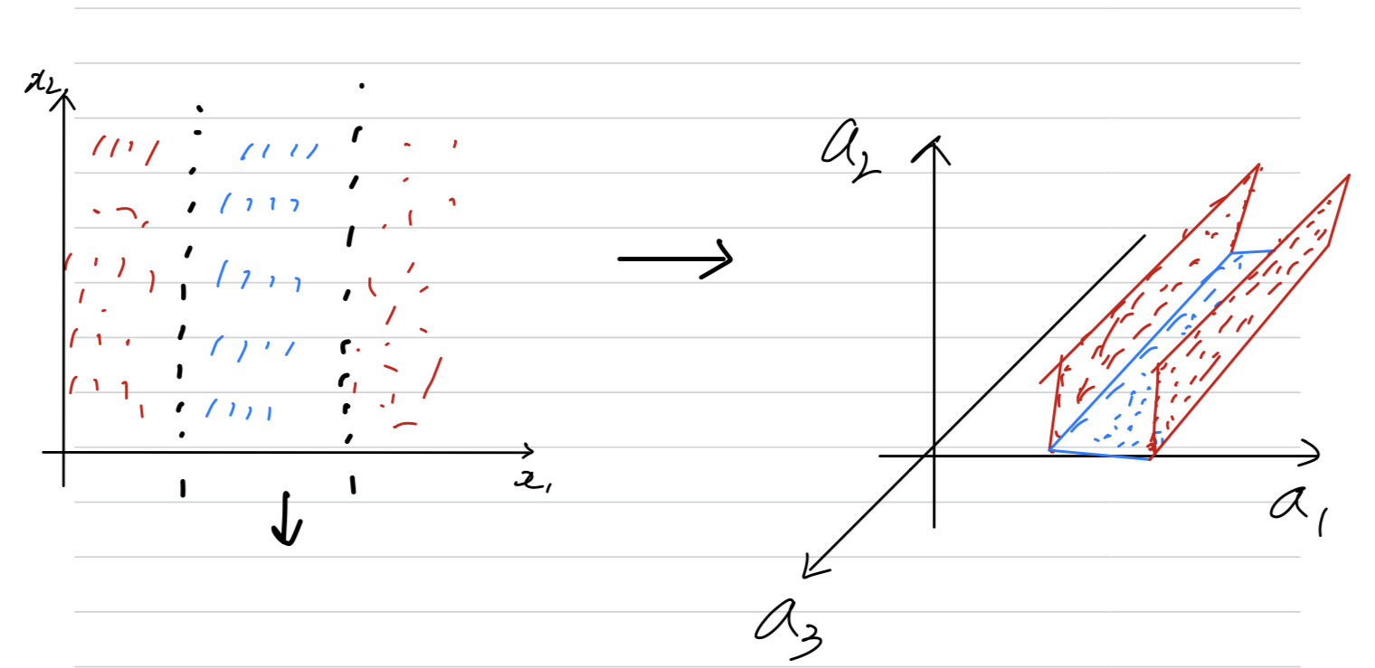
nonlinear function을 사용했는데 왜 직선으로 classification 되었을까?
- 아래 그림에서 hidden layer의 unit수가 4개이다.
만약 3개라고 가정했을 때,
2차원의 input feature가 nonlinear activation function을 거치며 3차원이 되었다.
따라서 data는 3차원에 존재하게 된다. (= 공간이 휘어졌다.)
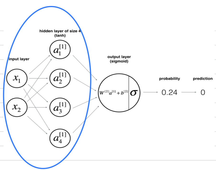
따라서 위, 위의 그림은 input feature들이 실제로 2차원에 존재하는 것이 아니라
hidden layer unit수가 이라고 하면, 차원에 존재하는 것인데 plotting을 2차원에 한 것일 뿐이다.
따라서 기존 2차원 일때는 직선 1개로 classification의 한계가 있었지만
3차원으로 바뀌면서 면 하나로 빨간 data와 파란 data를 classification할 수 있게 된다.
이러한 원리로 unit수를 늘리고, nonlinear activation function을 사용한다면 train set에 대하여 더욱 똑똑한 neural network가 된다.
- 아래 그림에서 hidden layer의 unit수가 4개이다.
