Week 3 | Shallow Neural Networks | Shallow Neural Network
Neural Network Representation
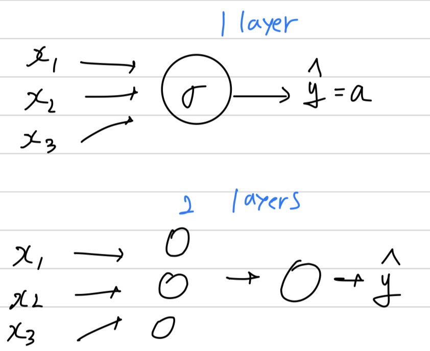
- We'll focus on the case of neural networks with what was called
a single hidden layer.
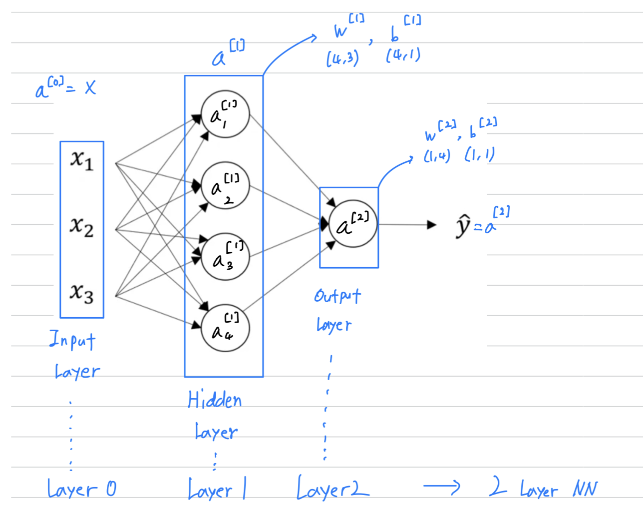
Input Layer = Layer 0:
Previously, we were using the vector to denote the input features.
Alternative notation for the values of the input features will be .
And the term also stands for activations, and it refers to the values that different layers of the neural network are passing on to the subsequent layers.
So the input layer passes on the value to the hidden layer,
so we're goting to call that activations of the input layer
Hidden Layer = Layer 1:
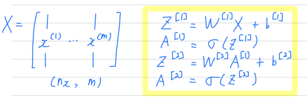
= []
(4, 1) column vectorOutput Layer = Layer 2:
the output layer regenerates some value which is just a real number.
is going to take on the value of
- technically there are 3 layers in this neural network
because there's the input layer, the hidden layer, the output layer.
But in conventional usage, if you read research papers and elsewhere in the course, you see people refer to this particular neural network as a 2 layer neural network,
because we don't count the input layer as an official layer.
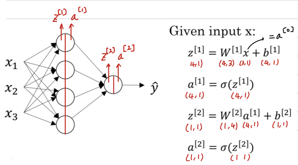
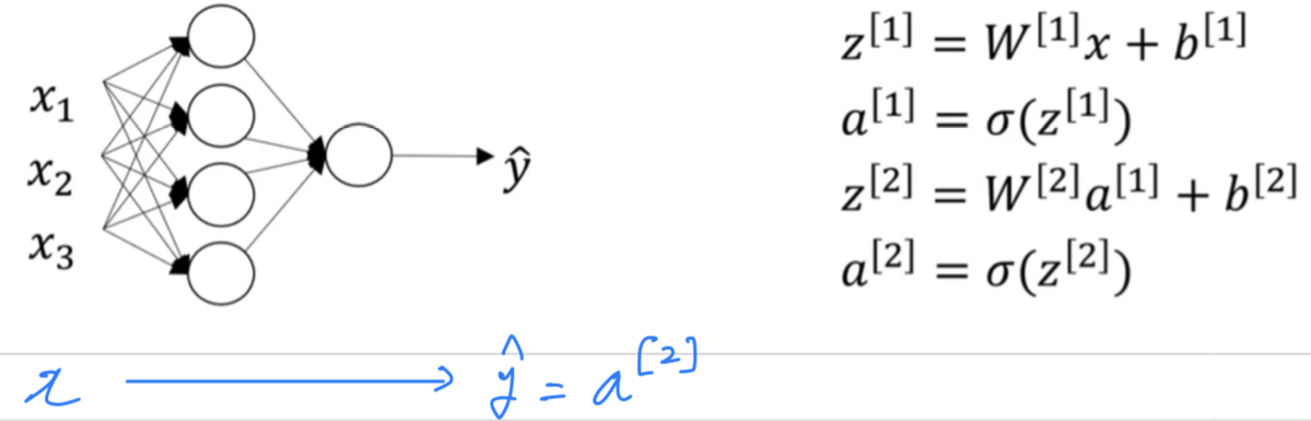
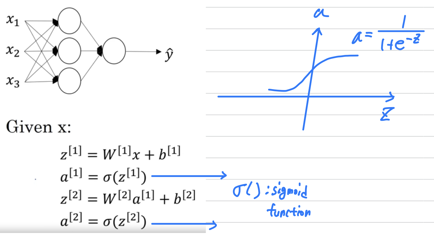
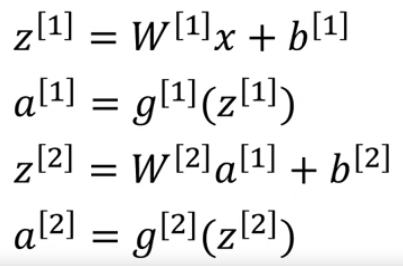
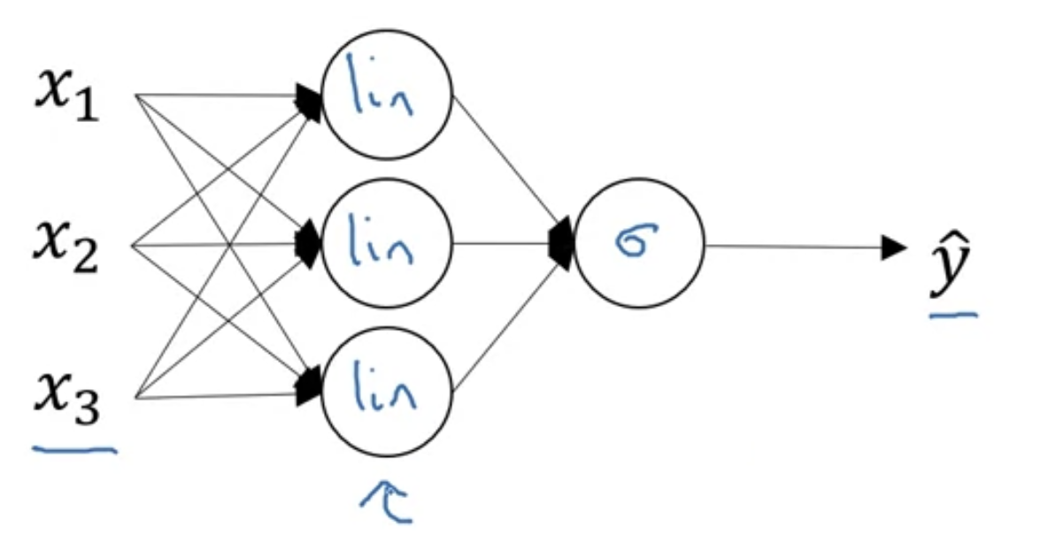
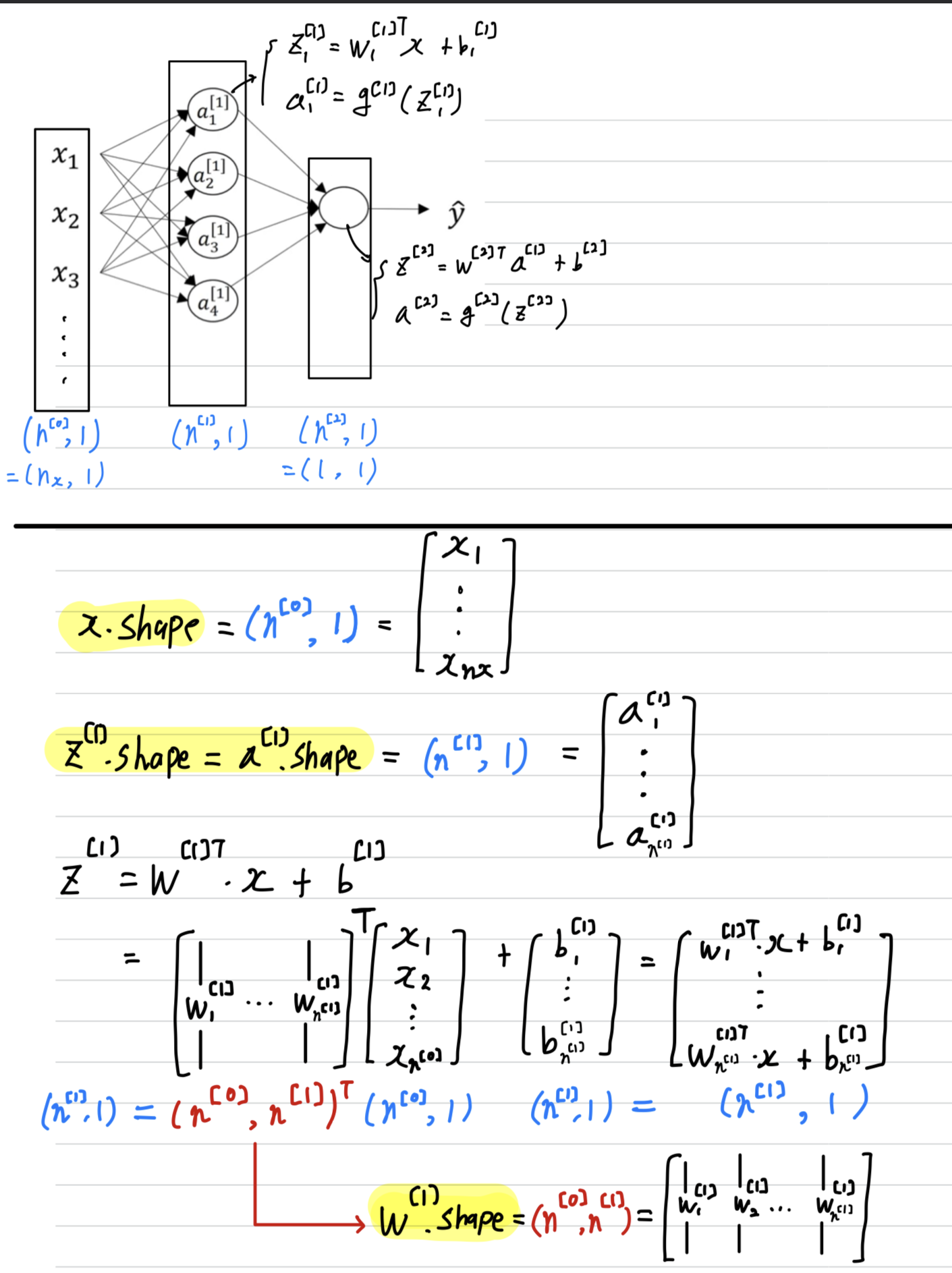
Computing a Neural Network's Output
-
The circle in logistic regression really represents two steps of computation rows.
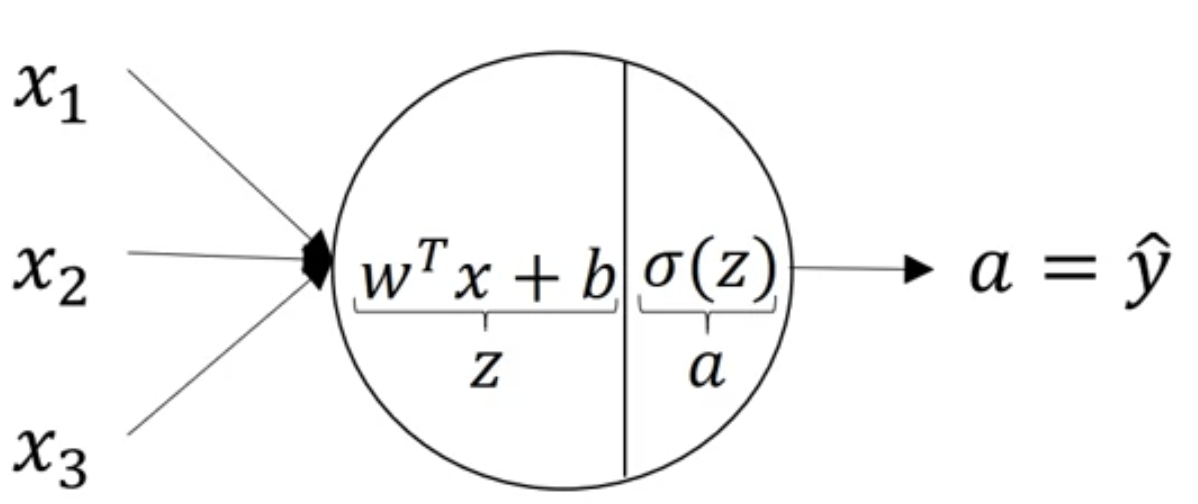
-
A neural network just does this a lot more times.
Let's start by focusing on just one of the nodes in the hidden layer.
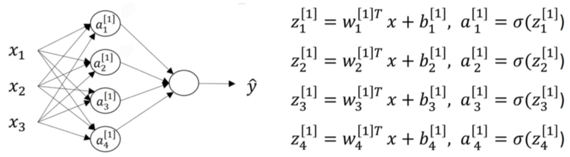
( : layer, : node in layer)-
Let's look at the first node in the hidden layer
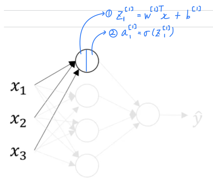
-
Let's look at the second node in the hidden layer
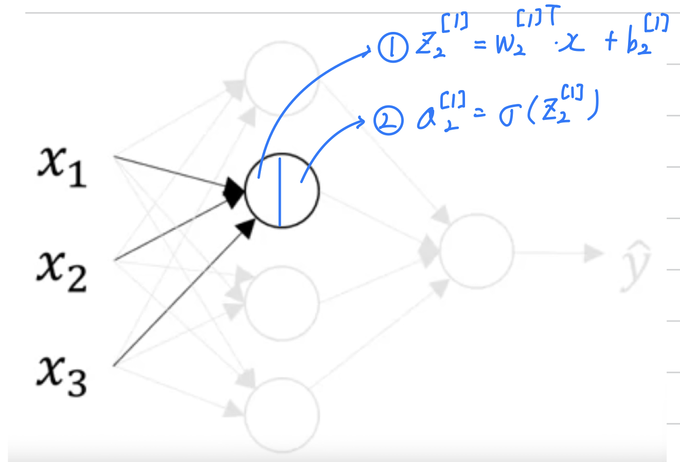
-
-
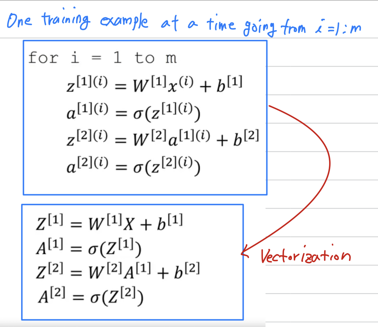
So, what we're going to do,
is take these four equations and vectorize.
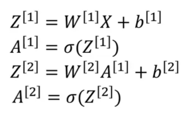
- we're going to start by showing how to compute as a vector
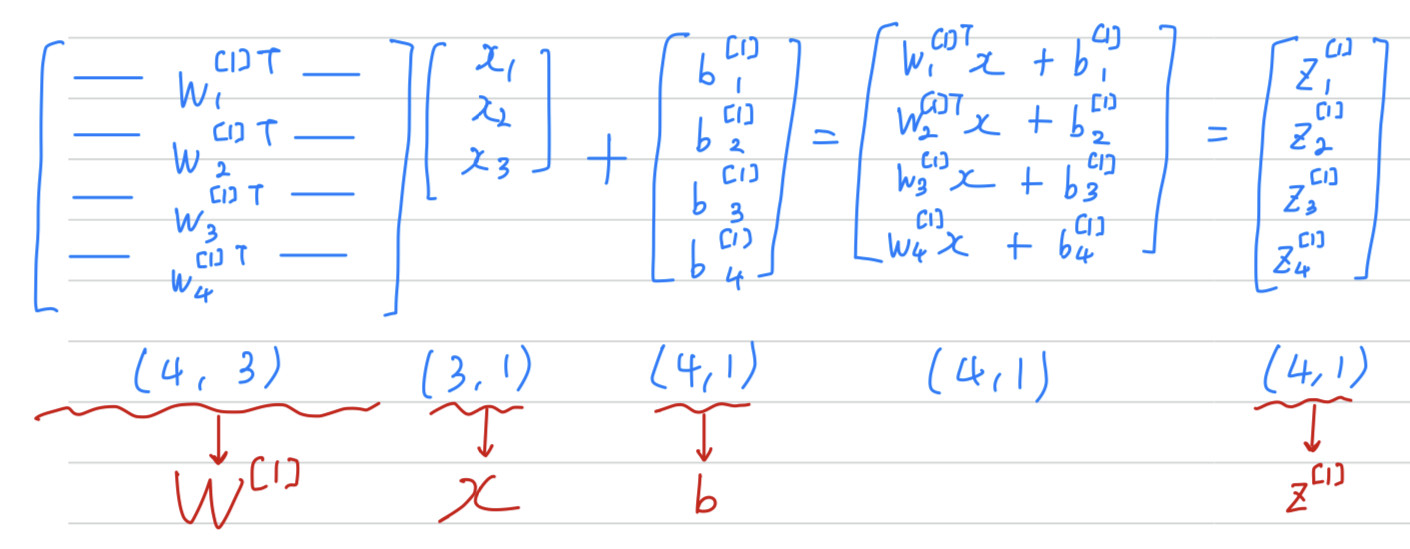
- Vectorized implementation of computing
- we're going to start by showing how to compute as a vector
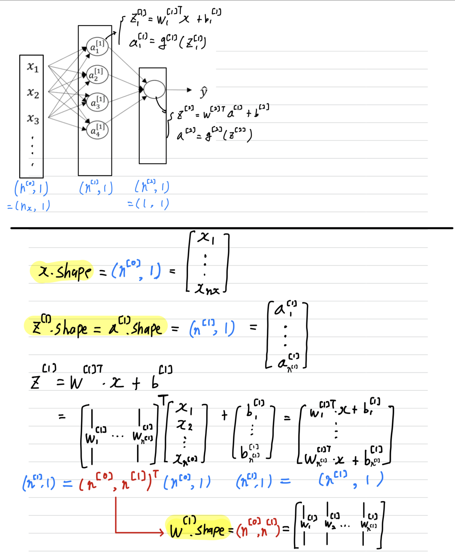
﹗Checking dimension (by myself)
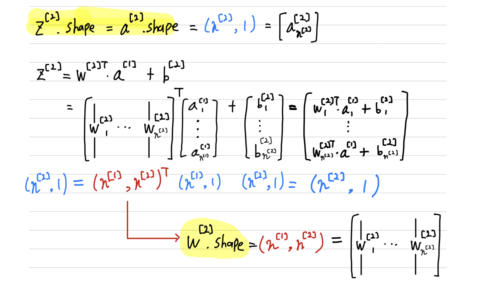
Vectorizing Across Multiple Examples
-
We can generate for a single training example.
-
We see how to vectorize across multiple training examples.
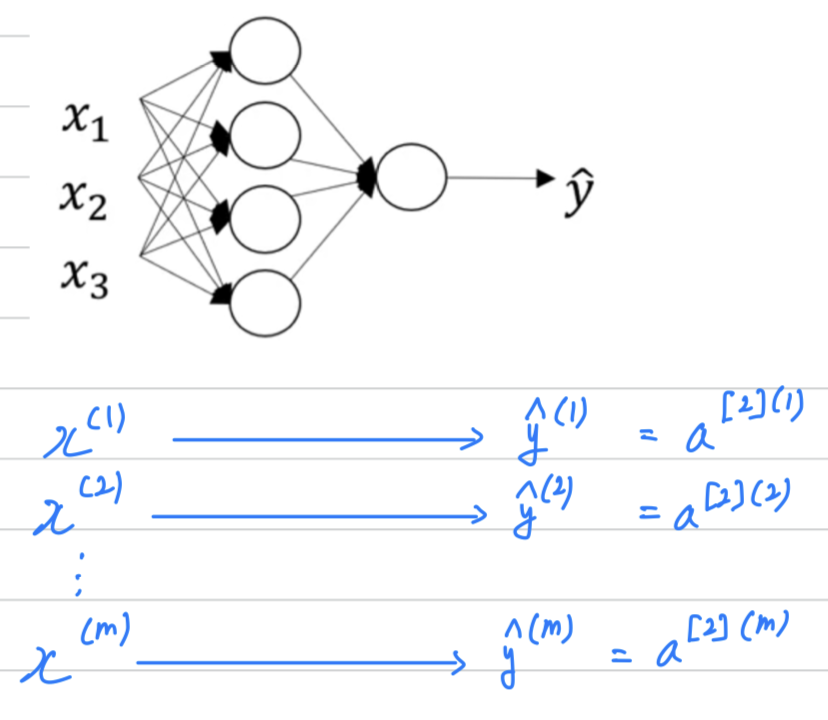
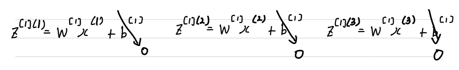
: Layer
: training example -
To suggest that if we have an
unvectorized implementationand
want to compute the predictions of all our trainin examples,
we need to do to
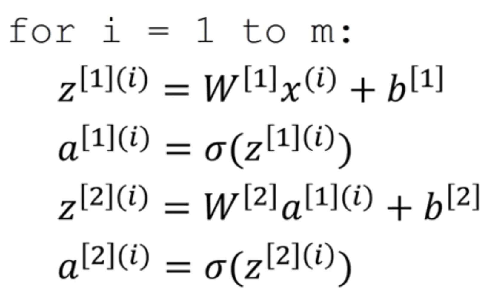
-
We'll see how to
vectorizethis.
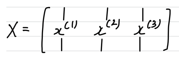
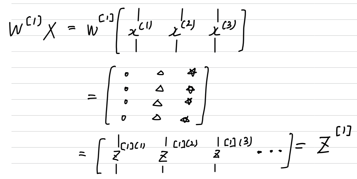
(we recall that we defined the matrix to be equal
to our training examples stacked up in these columns like so.
So this become a dimension of the matrix)
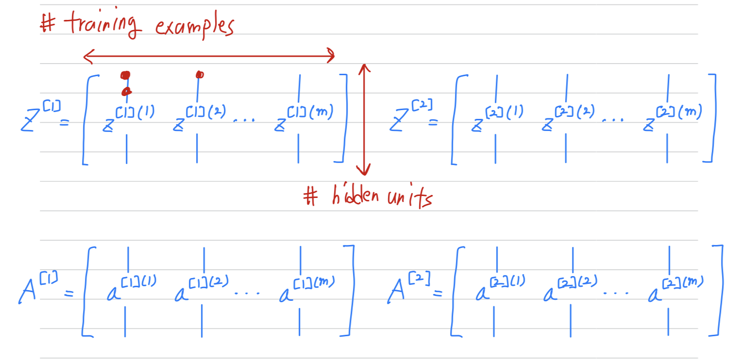
- The horizontally indices correspond to different training examples.
- The vertically indices correspond to different nodes in neural network.
- example :
matrix 의 가장 왼쪽 위 value :
the activation of the first hidden unit on the first training example을 의미.
matrix 의 가장 왼쪽 위의 한 칸 아래 value :
the activation of the second hidden unit on the first training example을 의미.
- example :
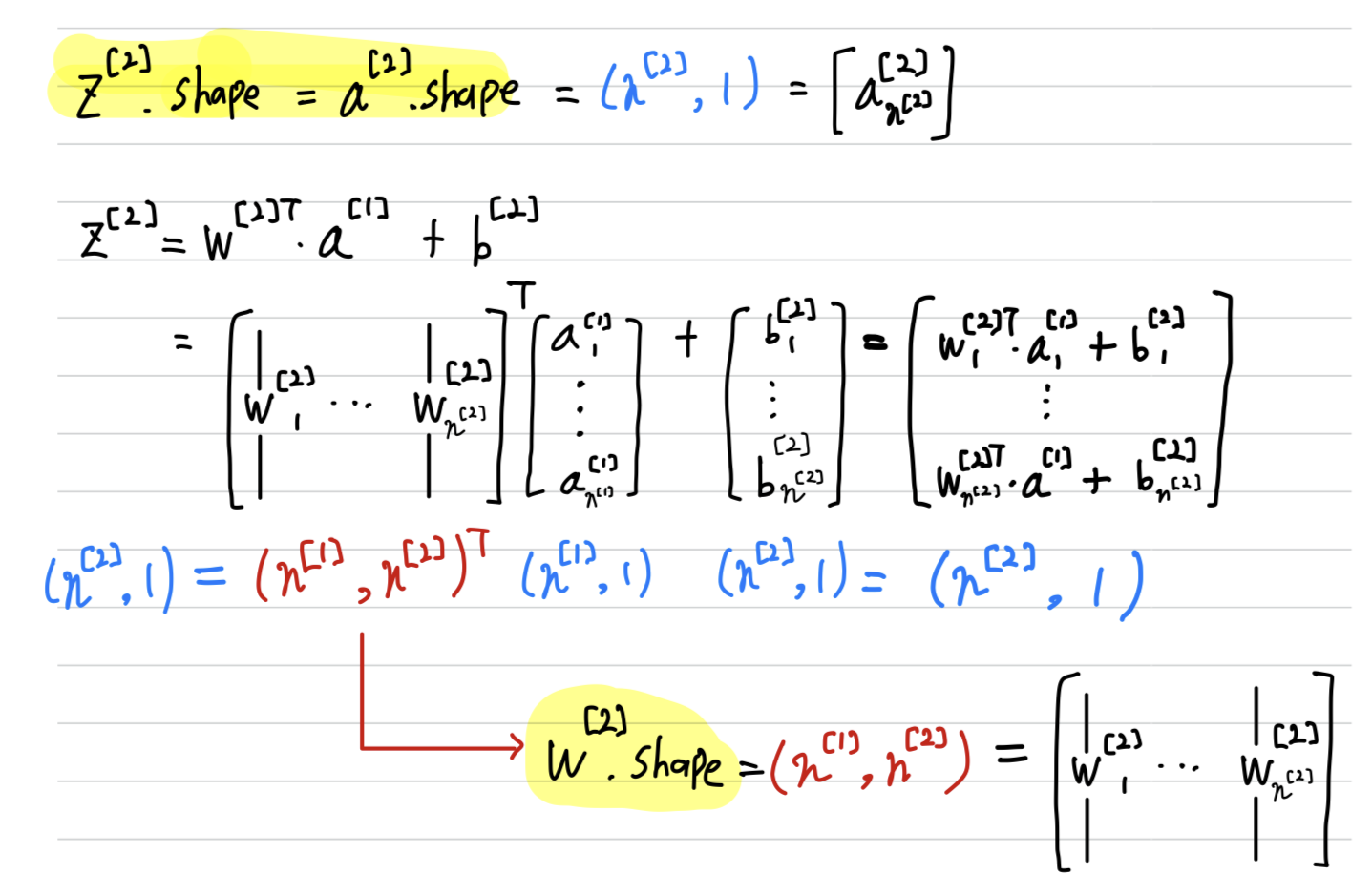
Checking dimension when vectorization(by myself)

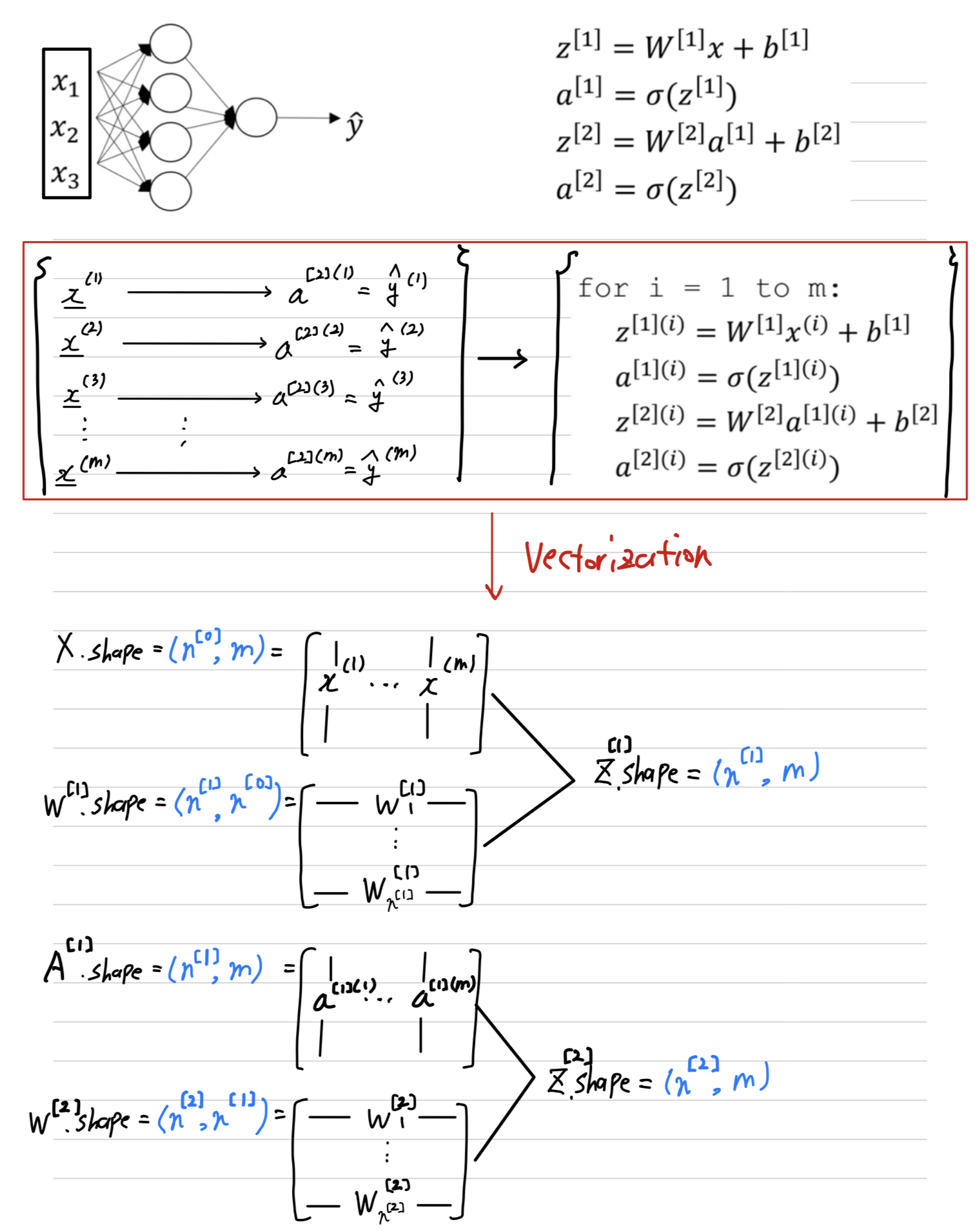
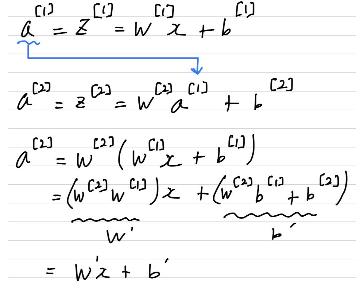
Explanation for Vectorized Implementation
- let's just say, to simplify this justificatino a little bit that is equal to
- Now, is going to be some matrix.
So if you look at this calculation , gives you some column vector which you must draw like this. (Similarly )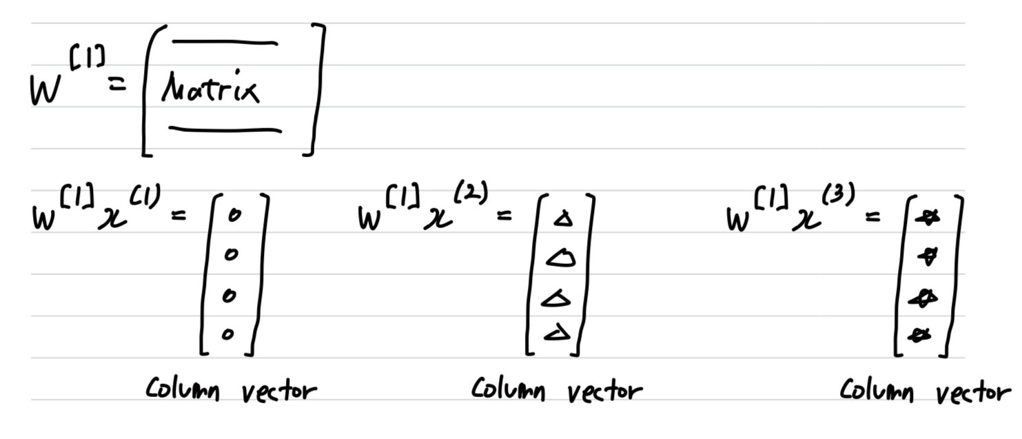
- So now, if you consider the training set , which we form by stacking together all of our training examples.
So the matrix is formed by taking the vector and stacking it vertically with and then also
- if you now take this matrix x and multiply it by w then you end up with,
Recap of vectorizing across multiple examples
- If this is our neural network,
- we said that this is what we need to do if we were to implement forward propagation,
one training example at a time going from euqal through .
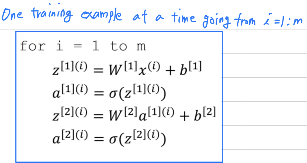
- And then we said,
Let's stack up the training examples in columns like so and for each of these values
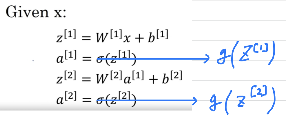
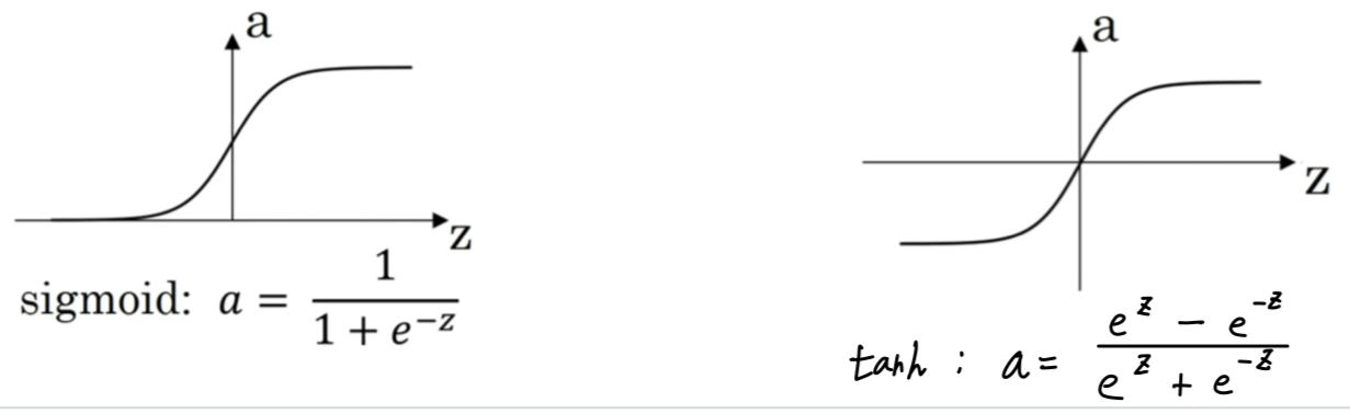
Activation Functions
-
So far, we've just been using the sigmoid function,
but sometimes other choices can work much better. -
In the forward propagation steps for the neural network,
we had these two steps where we use the sigmoid function here.
So that sigmoid is called an activation function.
-
So in the more general case,
we can have a different function
where could be anonlinear functionthat may not be the sigmoid function.
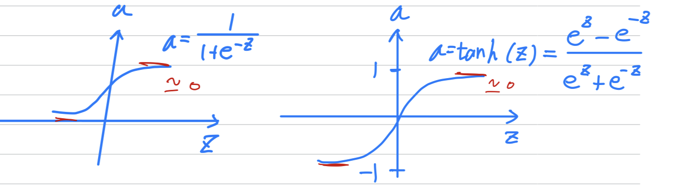
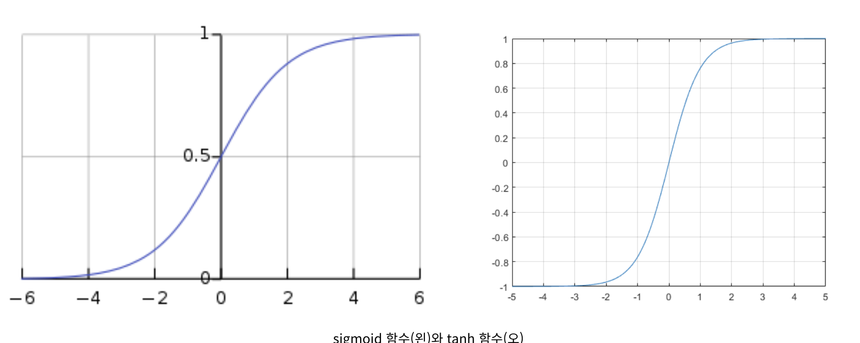
Hyperbolic Tangent : tanh
- So for example, the sigmoid function goes between and
An activation function that almost always works better than the sigmoid function is
the tangent functionorthe hyperbolic tangent function.
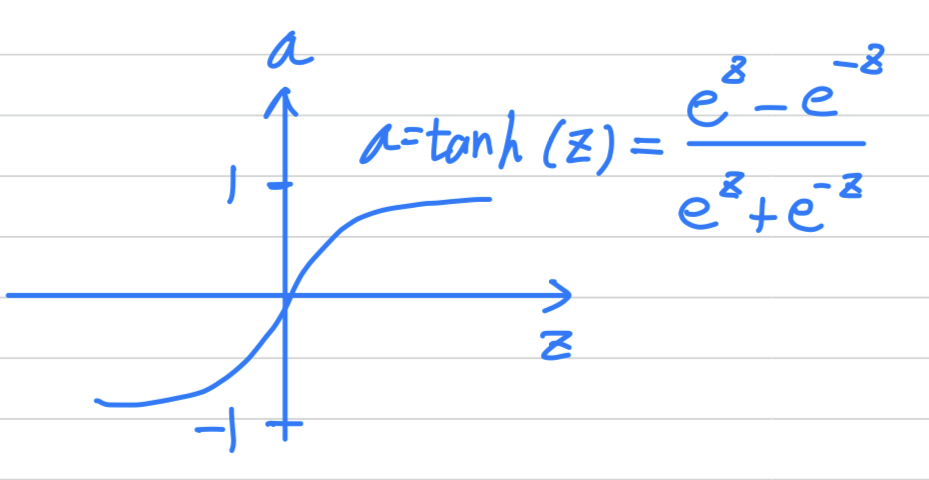
- The formula for the function is .
- It's actually mathematically a shifted version of the sigmoid function.
- This almost always works better than the sigmoid function because with values
between and ,
the mean of the activations that come out of ourhidden layerare closer to having a zero mean.
and so just as sometimes when we train a learning algorithm,
we might center the data and have our data have zero mean using a tanh instead of sigmoid function.
Kind of has the effect of centering our data so that the mean of our data is close to zero rather than maybe .
and this actually makes learning for the next layer a little bit easier. The one exceptionis for the ouptut layer because if is either or ,
then it makes sense for to be a number
that we want to output that's between and rather than between and .
So the one exception where we would use the sigomid activation function is when
we're using binary classification.
In which case we might use the sigmoid activation function for theoutput layer.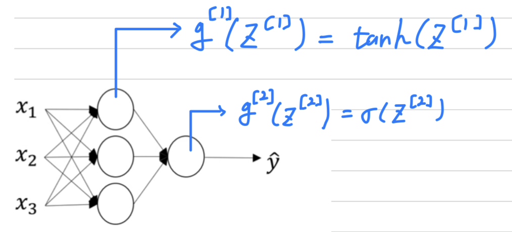
So what we see in this example is where
we might have a tanh activation function for the hidden layer and a sigmoid for the output layer.
So the activation functions can be different for different layers.
And sometimes to denote that the activation functions are different for different layers,
we might use square brackets superscripts as well to indicate that
g[1] may be different than g[2].
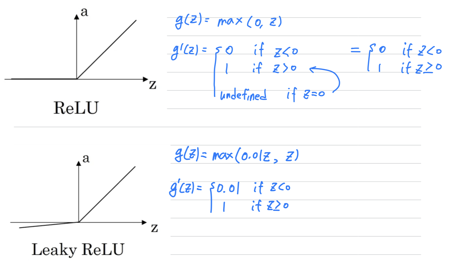
ReLU
-
One of the
downsidesof both the sigmoid function and tanh function is that
if is either very large or very small,
then the gradient of the derivative of the slope of this function becomes very small.
So if is very large or is very small,
the slope of the function either ends up being close to zero and so this can slow down gradient descent.
-
So one other choice that is very popular in machine learning is
what's called therectified linear unit.
So theReLUfunction looks like this and the formula is
So the derivative is so long as is positive and
derivative or the slope is when is negative.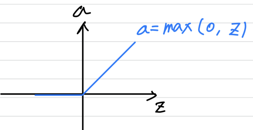
-
The fact that, so here's some rules of thumb for choosing activation functions.
- if your output is or value, if you're using binary classification,
then the sigmoid activation function is very natural choice for the output layer. - And then for all other units ReLU is increasingly the default choice of activation function.
So if you're not sure what to use for your hidden layer,
I would just use the ReLU activation function, is what you see most people using these days.
Although sometimes people also use the tanh activation function.
- if your output is or value, if you're using binary classification,
Leaky LeRU
- One disadvantage of the ReLU is that the derivative is equal to when is negative.
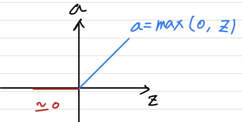
- In practice this works just fine
but there is another version of the ReLU called theLeaky ReLU.
Instead of being when is negative, it just takes a slight slope like so.
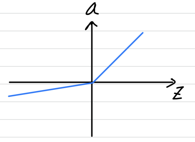
- This usually works better than the ReLU activation function.
Although, it's just not used as much in practice.
Either one should be fine. (둘 중 아무거나 사용해도 괜찮다.) - And the advantage of both the ReLU and the Leaky ReLU is that for
a lot of the space of , the derivative of the activation function,
the slope of the activation function is very different from .
And so in practice, using the ReLU activation function,
our neural network will often learn much faster than when using the tanh or the sigmoid activation function.
And the main reason is that there's less of this effect of slope of the function going to , which slows down learning.
- This usually works better than the ReLU activation function.
Pros and cons of activation functions
-
sigmoid function&tanh function:
I would say never usesigmoid functinoexcept for the output layer
if you're doing binary classification or maybe almost never us this.
I almost never use this because thetanh functionis pretty much strictly superior.
-
ReLU:
The most commonly used activation function isReLU.
So if you're not sure what else to use, use this one.
And maybe, feel free also to try theLeaky ReLU
(why is that constant 0.01? You can also make that another parameter of the learning algorithm.
And you can just see how it works and how well it works, and stick with it if it gives you a good result)
One of the things we'll see in deep learning is that
you often have a lot of different choices in how you build your neural network.
Raning from a number of hidden units to the choices activation function, to how you initialize the ways...
And it turns out that it is sometimes difficult to get good guildelines
for exactly what will work best for your problem.
If you're not sure which one of these activation functions work best, try them all.
And evaluate on like a holdout validation set or like a development set.
And see which one works better and then go of that.
Why do you need Non-linear Activation Functions?
-
Why does a neural network need a non-linear activation function?
-
So, here's the forward prop equations for the neural network.
-
Why don't we just get rid of the function and set equals ?
➡️ we can say that
Sometimes this is called the linear activation function.
(a better name for it would be the identity activation function)
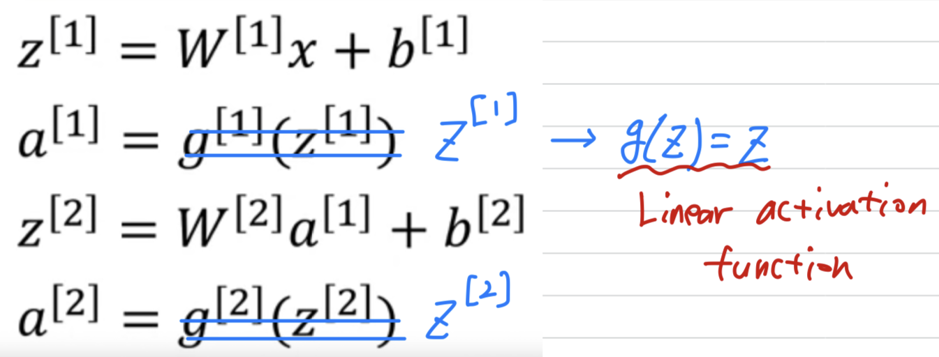
 ➡️ if you were to use linear activation functions or we can also call them identity activation functions,
then the neural network is just outputting a linear function of the input.
➡️ And we'll talk about deep networks later, neural networks with many, many hidden layers.
And it turns out that if you use a linear activation function or alternatively,
if you don't have an activation function, then no matter how many layers your neural networks has,
all it's doing is just computing a linear activation function.
So you might as well not have any hidden layers.
 ➡️ But the take home is that a linear hidden layer is more or less useless
because the composition of two linear functions is itselft a linear function.
그래서 만약 저 곳에 non-linear function을 사용하지 않는다면,
network가 깊어질수록 더 많은 computing을 할 수 없게 된다. -
There is just one place where you might use a linear activation function .
And that's if you are doing machine learning on the regression problem.
So if is a real number.-
So for example, if you're trying to predict housing prices.
So is not , but is a real number, anywhere from $ ~ $
Then it might be okay to have a linear activation function here
so that your output is also a real number going anywhere from toBut then the hidden units should not use the activation functions.
They could use ReLU or tanh or Leaky ReLU or maybe something else.
So the one place you might use a linear activation funcion is usually in the output layer.
But other than that, using a linear activation function in the hidden layer
except for some very special circumstances relating to compression that we're goint to talk about using the linear activation function is extremely rare.And, of course, if we're actually predicting housing prices,
because housing prices are all non-negative, perhaps even then you can use a ReLU activation function so that your output are all greater than or euql to 0
-
-
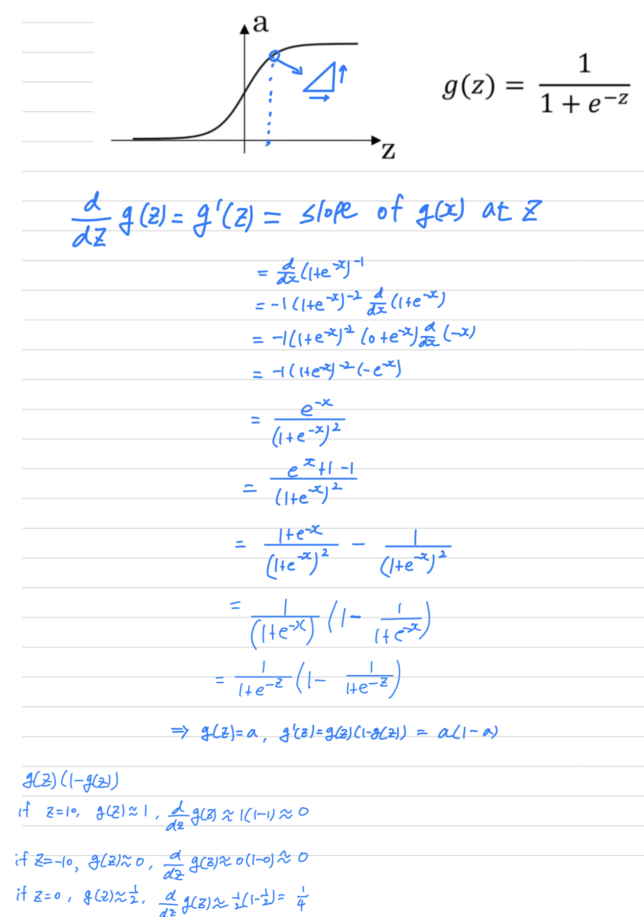
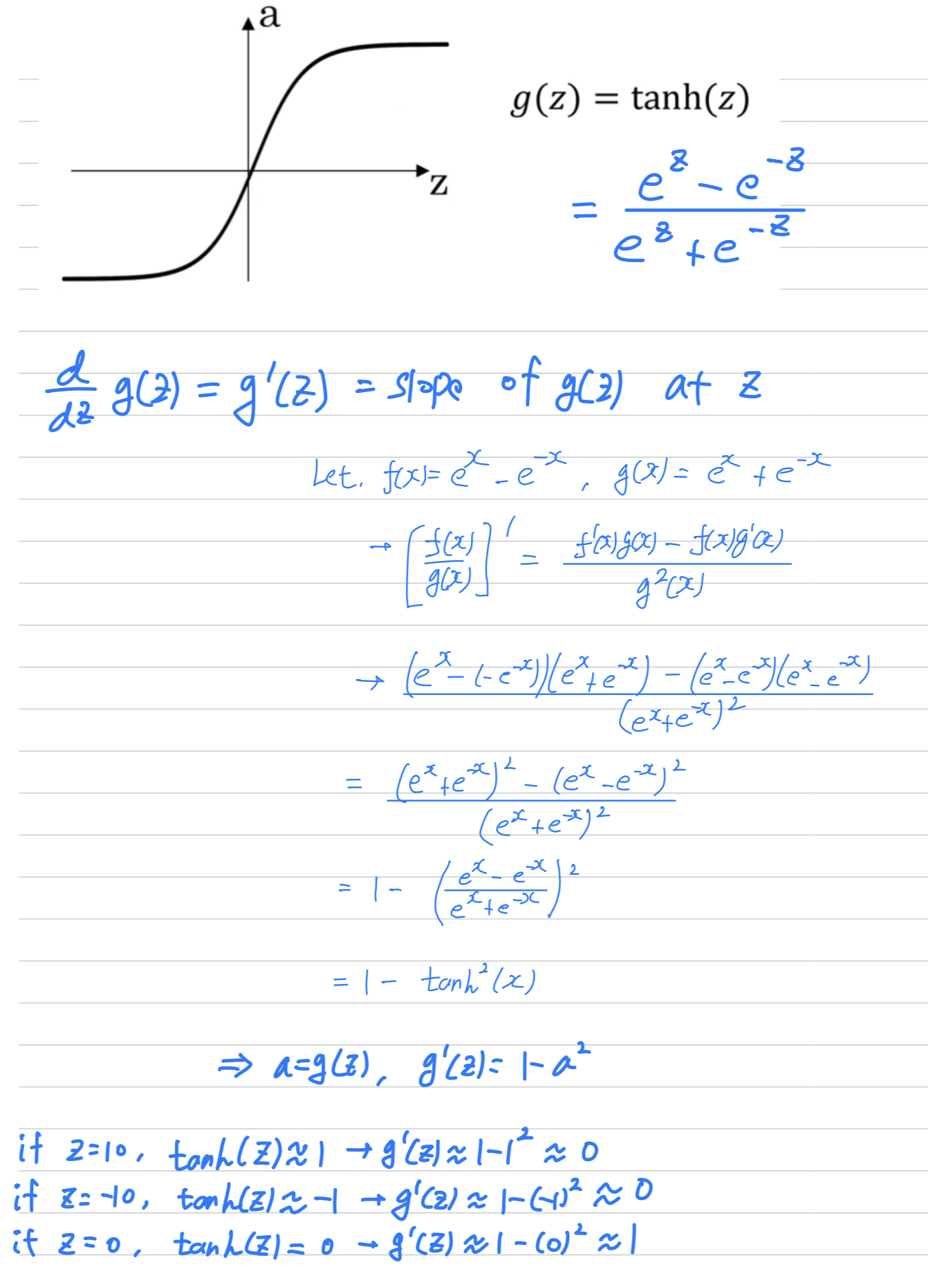
Derivatives of Activation Functions
sigmoid activation function
Tanh activation function
ReLU and Leaky ReLU
- it's actually undefined, technically undefined if
But if you're implementing this in software, it might not be a 100 percent mathematically correct,
set the derivative to be equal to .
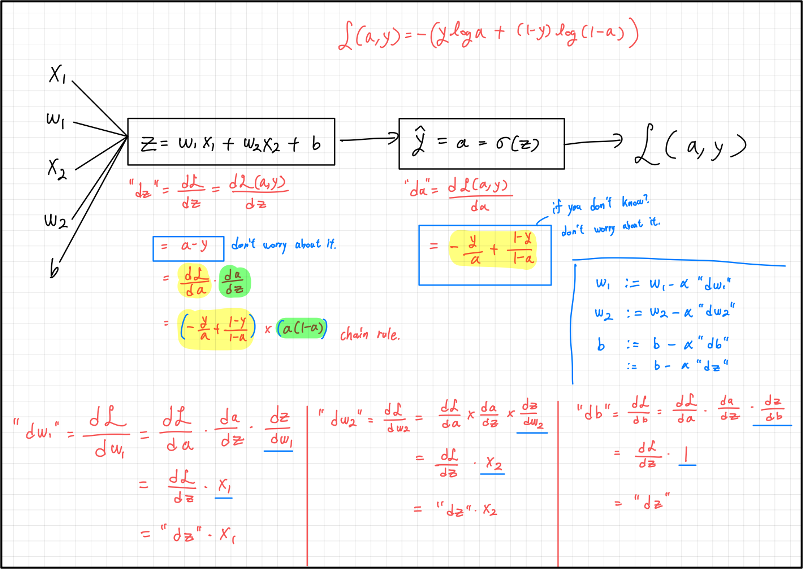
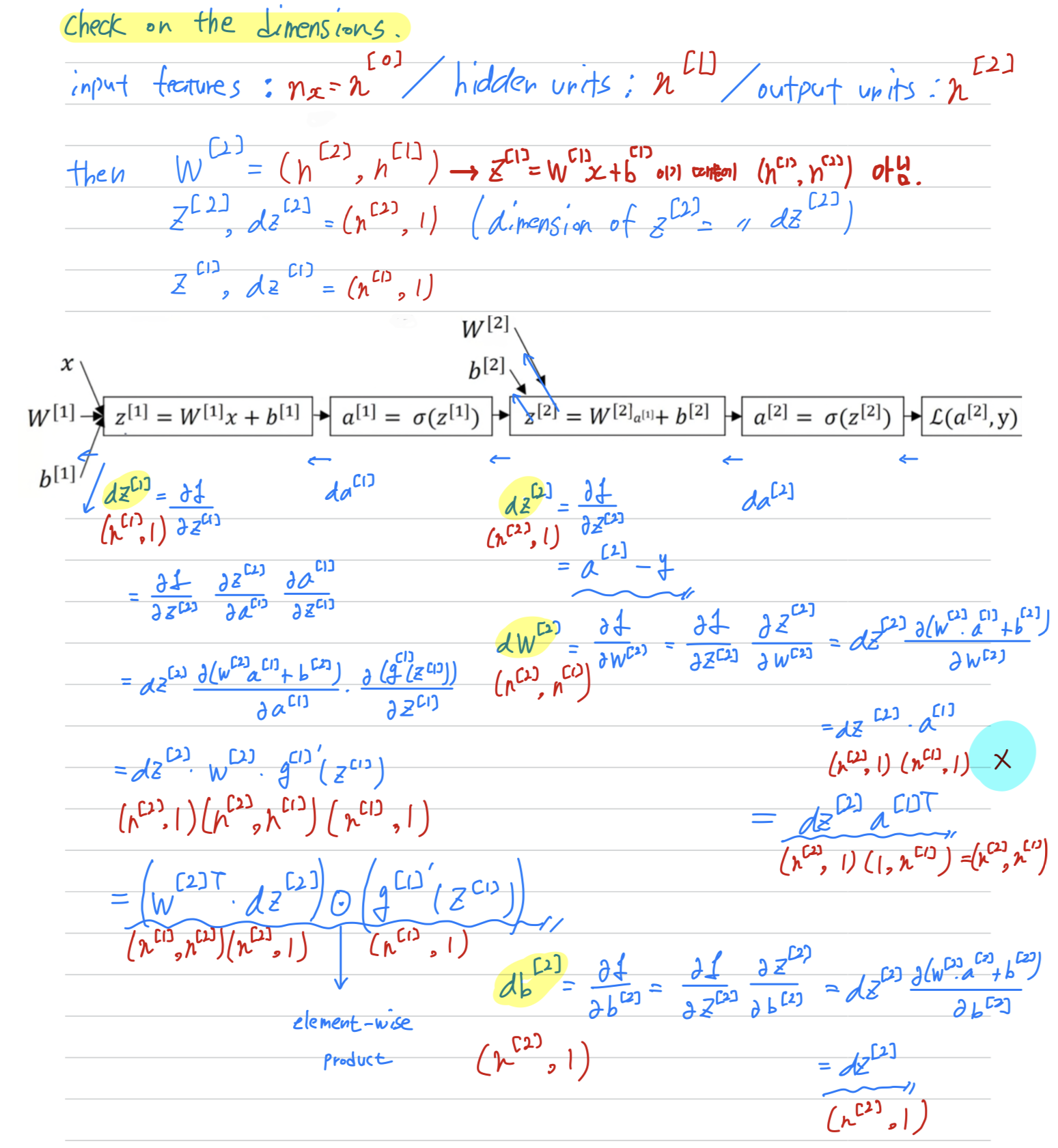
Gradient Descent for Neural Networks
-
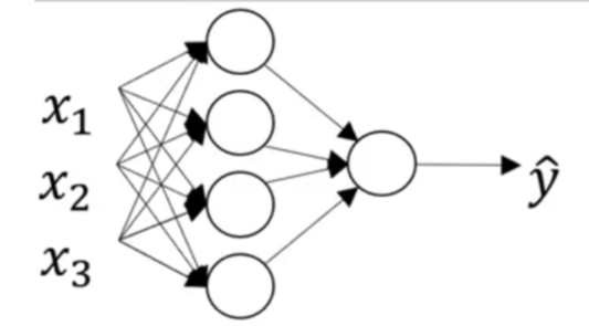
Our neural network with a single hidden layer for now, will have
parameters
(you have input features, and hidden units, and output units)
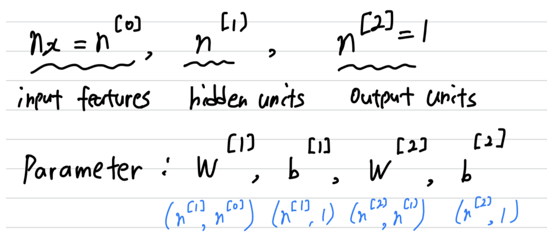
-
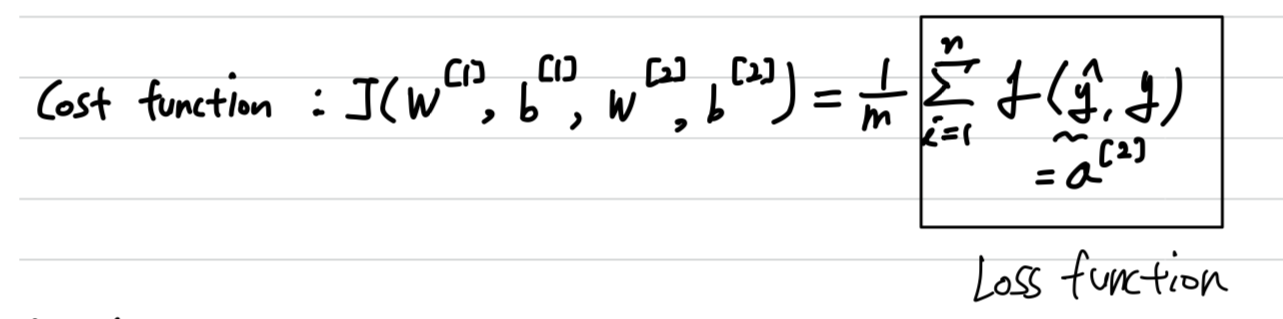
We also have
cost functionfor a neural network.
For now, we'are just going to assume that we're doing binary classification.
-
To train parameters of our algorithm, we need to perform
gradient desent.
When training a nerual netowork, it is important to initialize the parameters randomly rather than to all zeros.
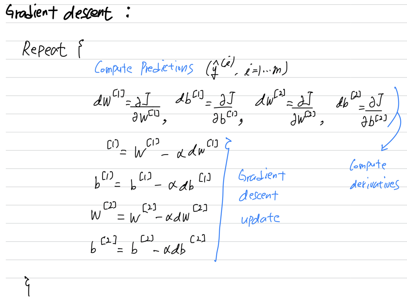
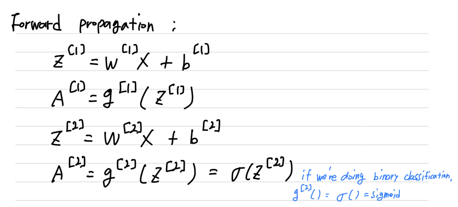
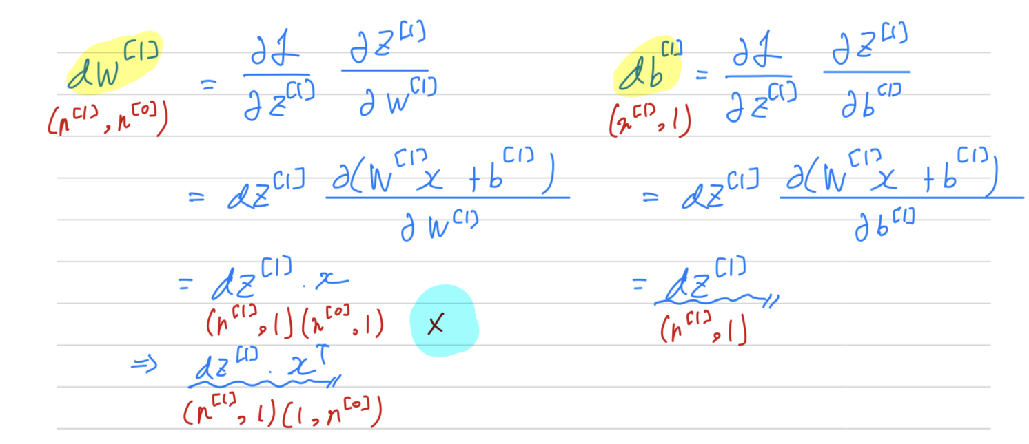
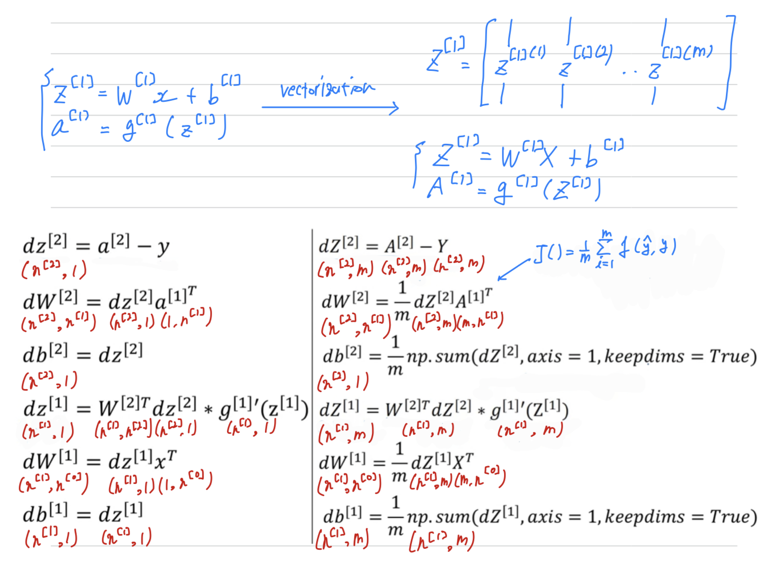
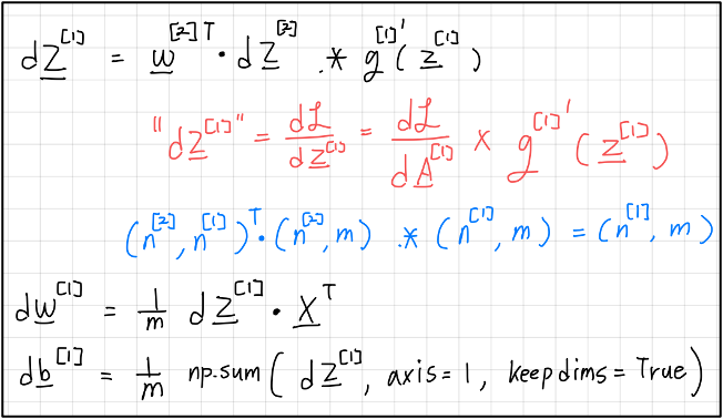
Formulas for computing derivatives
forward propagation
- Let me just summarize again the equations for forward propagation.
back propagation
- Next, let's compute the derivatives.
So, this is the back propagation step.- Recall about logistic regression
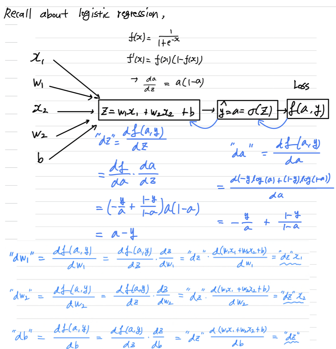
- Now we have not going to an output unit,
but going to a hidden layer and then going to an output unit.
Instead of this computation, beging 1 step, we'll have 2 steps in this neural network with 2 layers
- So in this 2 layers neural network, that is with the input layer, hidden layer, and an output layer.
(One tip when implementing backprop,
if you just make sure that the dimensions of your matrices match up,
if you think through, what are the dimensions of your various matrices
including , and so on
and just make sure that the dimensions of theses matrix operations may match up,
sometimes that will already eliminate quite a lot of bugs in backprop.)

- Recall about logistic regression
Summary of gradient descent (Vectorization)
Random Initialization
-
it's important to initialize the weights randomly.
For logistic regression, it was okay to initialize the weights to zero.
But for a neural network of initialize the weights to parameters to all zero and
then applied gradient descent, it won't work.
Let's see why. -
So it's possible to construct a proof by induction that
if you initialize all the values ,
then because both hidden units start off computing the same function,
and both hidden units have the same influence on the output unit,
then after one iteration, that same statement is still true,
the two hidden units are still symmetric.
And therefore, after two iterations, three iterations and so on,
no matter how long you train you neural network,
both hidden units are still computing exactly the same function.
And so in this case, there's really no point to having more than one hidden unit.
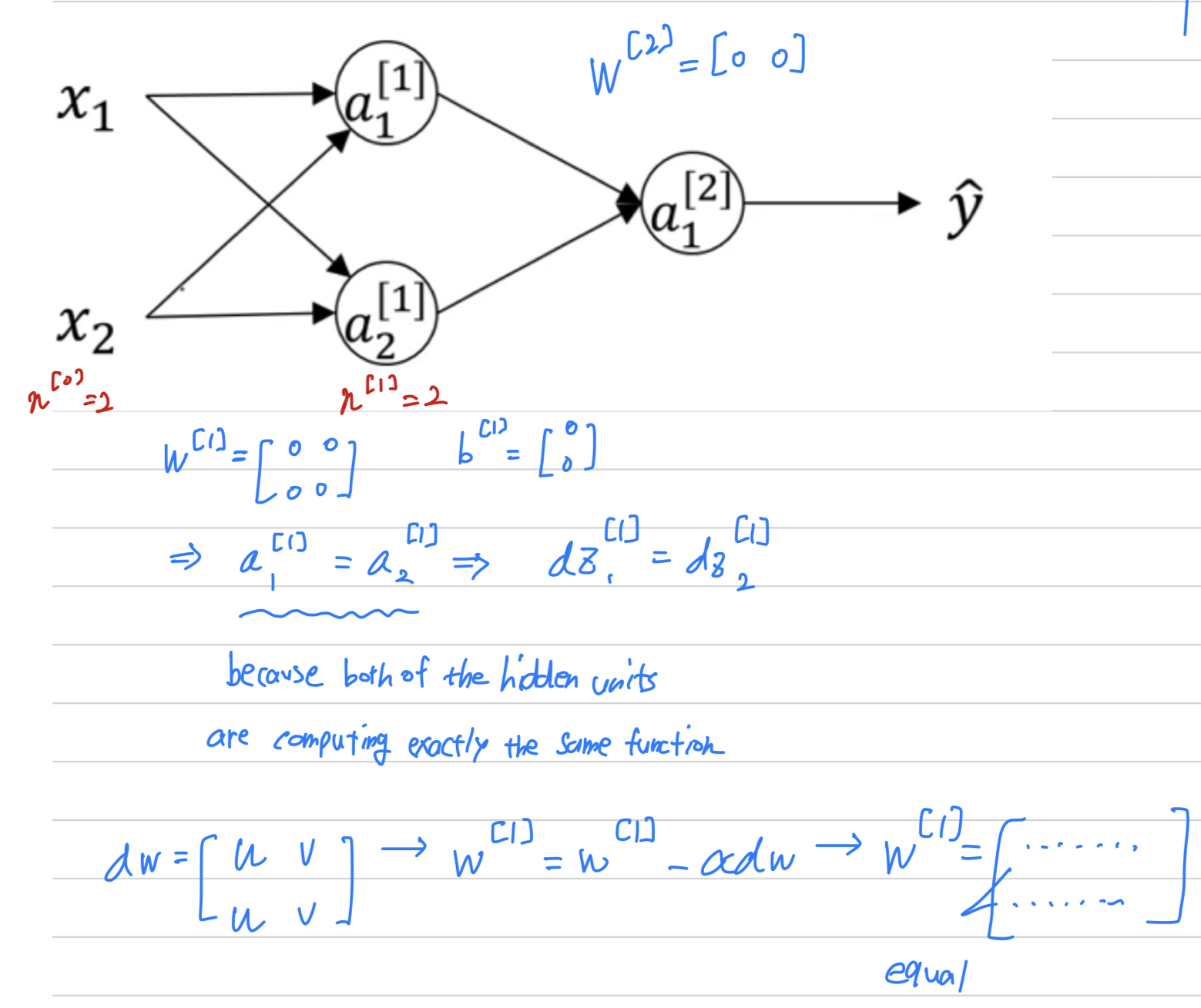
-
The solution to this is to initialize your parameters randomly.
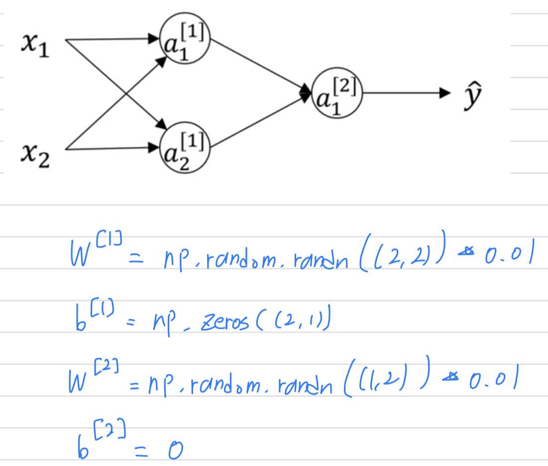
- it's okay to initialize to zeros.
Because so long as is initialized randomly,
you start off with the different hidden units computing different things.
And so you no longer have this symmetry breaking problem.) - Wht not put the number 100 or 1000 instead of 0.01?
Because if you are using a tanh or sigmoid activation function,
or the other sigmoid, even just at the output layer.
If the weights are too large, then when you compute the activation values,
remember that
and then
So if is very big, will be very, or at least some values of will be either very large or very small.
And so in that case,
you're more likely to end up at the fat parts of the tanh function or the sigmoid function,
where the slope or the gradient is very small.
Meaning that gradient descent will be very slow.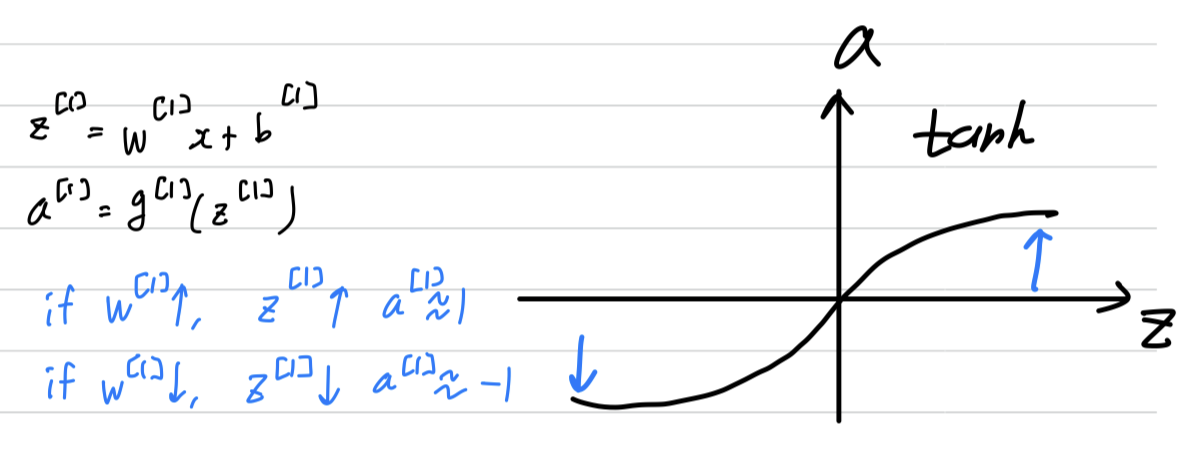
- it's okay to initialize to zeros.
Quiz
Semina - discussion
-
h5py :
HDF5는 binary data format이며,
h5py는 HDF5에 대한 pythonic interface를 제공하는 Package이다. -
logistic regression하기 전에, data를 preprocessing할 때, standardization하는 이유?
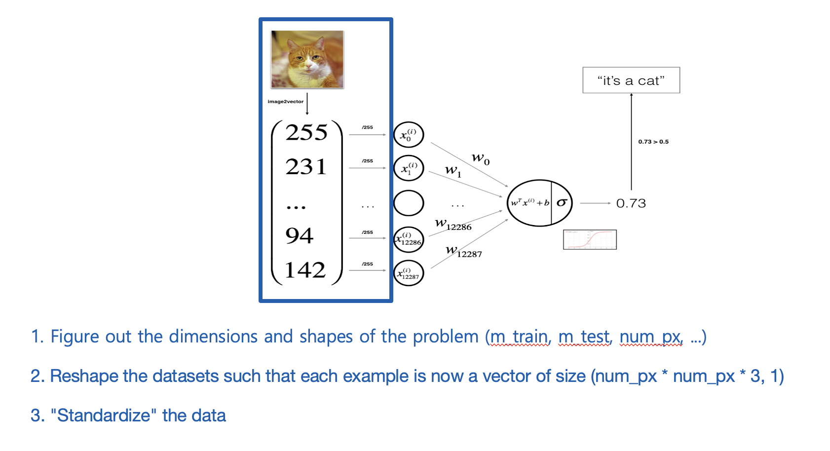
- 에서 값을 0~1 사이로 조정함으로써 값을 줄일 수 있다.
값을 줄이면, sigmoid(z)에서 기울기가 0인 부분보다 기울기가 더 큰 부분을 가리킬 수 있기 때문에 학습에 있어서 속도가 빠르다. - 또한 feature들이 여러 개라면, feature들 간의 scale조정이 필요하다.
만약 키, 몸무게라는 feature가 있다면, 두 feature 간의 scale 차이가 심하기 때문에 이를 0~1 사이의 값으로 조정해준다.
- 에서 값을 0~1 사이로 조정함으로써 값을 줄일 수 있다.
-
왜 hidden layaer에 nonlinear activation function만을 사용해야 할까?
linear activation function을 사용한다면
예를 들어 의 activation function을 사용한다고 가정하자.
그렇다면, 1 hidden layer를 지났을 때, 가 된다.
2 hidden layer를 지났을 때, 가 된다.
3 hidden layer를 지났을 때, 가 된다.
하지만 이처럼 3 hidden layer를 만들지 않고도 를 activation function 를 사용한 하나의 hidden layer로 만들 수 있다.
따라서, 3개의 hidden layer를 구성할 이유가 없어지는 것이다.
또한 linear activation function을 사용하면, 각 unit들도 모두 linear하기 때문에 prediction value도 linear하게 되고, 이는 no more expression하다.
따라서 nonlinear activation function을 사용함으로써 input feature 에 대한 변칙적인 계산을 수행하여 에 대해 더 많은 expression을 추출하여 좋은 prediction value를 만들 수 있게 해야 한다. -
zero initialization보다 Random initialization이 필요한 이유?
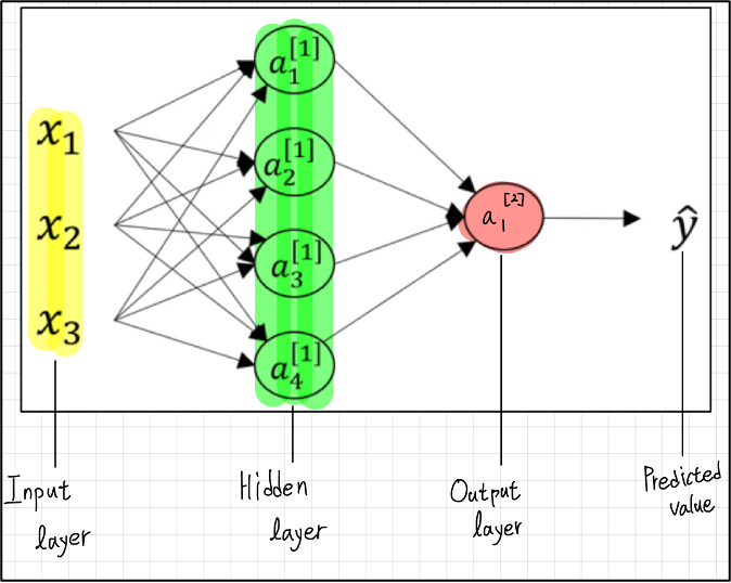 만약 모든 weight가 로 initialization된다면,
hidden layer의 모든 unit은 똑같은 computation을 할 것이다.
(이기 때문에)
위의 neural network에서는 hidden layer가 1개이고, 4개의 unit이 있다.
만약 backward propagation 과정에서 weight update값을 구할 때,
모두 같은 값으로 update되어 모든 weight가 계속 같은 값을 갖고 있을 것이다.
그렇다면 4개의 unit은 또 모두 동일한 computation을 수행하기 때문에,
4개의 unit의 computation은 1개의 unit의 computation과 똑같은 기능을 수행할 것이다.
따라서 weight를 initialization하면, learning이 이루어지긴 하지만 unit이 여러 개 있는 neural network의 기능을 기대하기 힘들 것이다.
따라서 weight를 initialization을 하여, unit 4개 각각이 서로 다른 computation을 통해 neural network 기능을 기대할 수 있다. -
sigmoid, tanh를 hidden layer의 activation function으로 사용하는 것보다 ReLU를 사용하는 것이 더 좋을까?
위 은 backward propagation과정에서 구하는 값이다.
을 구할 때, 을 구해야 한다.
만약 우리가 를 sigmoid 또는 tanh를 사용했다면,
sigmoid 또는 tanh의 derivative를 구해야 할 것이다.
하지만, sigmoid또는 tanh의 derivative를 구할 때, 학습에 치명적인 단점이 존재한다.
sigmoid와 tanh에 적용되는 축 value가 작거나 크면, derivative는 으로 수렴하게 된다.
sigmoid와 tanh의 derivative가 0으로 수렴한다는 의미는
으로 수렴한다는 의미가 되고,
과 값은 모두 의 곱셈연산이 적용되기 때문에
과 값도 모두 으로 수렴할 것이다.
그렇게 된다면, gradient descent를 수행할 때, 과 는 update가 되지 않거나, 매우 작은 값으로 update가 될 것이다.
이는 Learning이 일어나지 않는다는 의미가 된다.
따라서 activation function의 derivative가 0이 되는 구간이 없는 activation function인 ReLU함수가 이러한 면에서 더욱 장점을 갖는다.
또한 ReLU는 derivative를 구하기도 매우 간단하다.
- 다음의 backward propagation 과정의 에서 element-wise product를 하는 이유?
가 로 된 것이므로
가 어떠한 의미인지 살펴보자.
forward propagation 과정에서,
에 activation function인 을 적용하여 이 만들어졌다.
에 을 적용할 때, 모든 unit은 element-wise 연산으로 적용이 되었다.
따라서 를 구할 때도 element-wise로 각 unit마다 update해야 하는 값을 구해야 하기 때문에
에서 을 element-wise product로 수행하는 것이다.
