Invariant descriptors

scale invariant

• scale에 invariant한 descriptor를 찾아볼 것이다.
  이러한 상황에서 한가지 방법으로는 rescale the patch

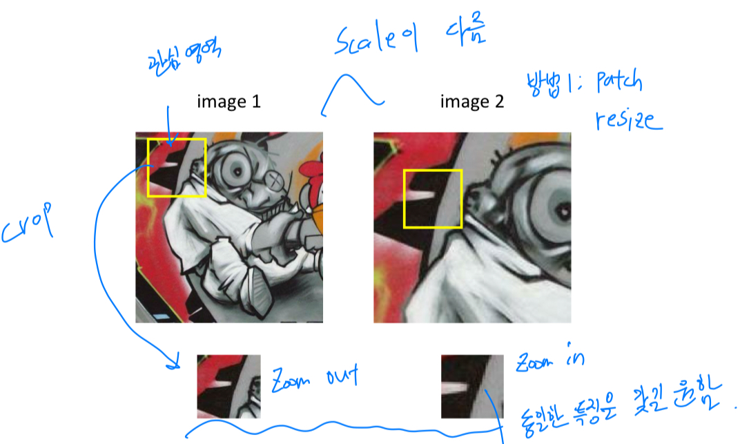
possible solution 1 : rescale the patch

• rescale the patch : crop하는 영역의 크기를 다르게 한다.
  
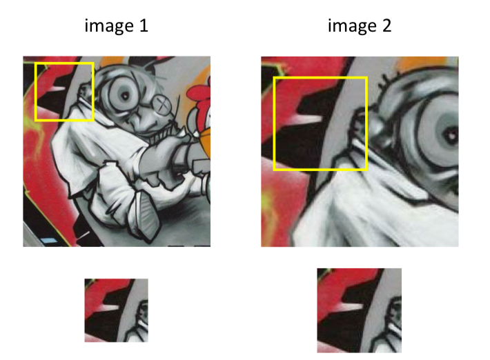
• 하지만, 이렇게 scale을 바꿔가는 과정은 exhuastive search이다.
  complexity : $O(N^2)$
• 따라서 scale selection 과정을 자동화하길 원한다. = automatic scale selection

solution : automatic scale selection

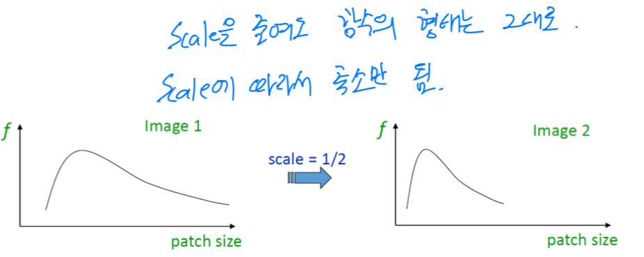
• automatic scale selection :
  patch들의 scale이 다르더라도 대응되는 값이 갖도록 하는 함수를 design하는 것.
  

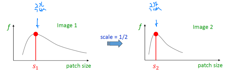
• 극값(local maxima, local minima)을 이용하여 얼만큼 scaling할 것인지 판단할 수 있다.
  

• patch의 scaling이 커짐에 따라서 각각의 image에 적합한 scale을 찾을 수 있다
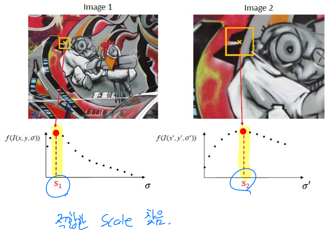  적합한 scale이 찾아지면,
  해당 patch를 우리가 알고 있는 일반적인 좌표(canonical size)로 갖고 와서 normalization하고,
  그 상태에서 feature를 추출하면, scale에 invariant한 feature를 추출할 수 있음

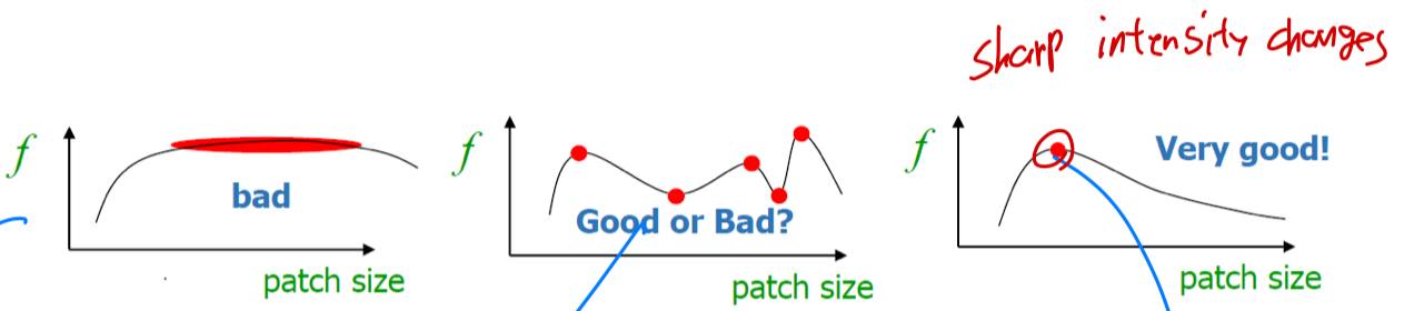
• 적합한 patch size가 넓은 구간에 걸쳐서 존재하는 것보다 stable하면서 sharp한 peak를 갖는 것이 적합한 함수로 여겨진다.
  

• 그렇다면 peak점을 어떻게 찾을까?
  edge를 찾는 kernel을 convolution시킨다.
  
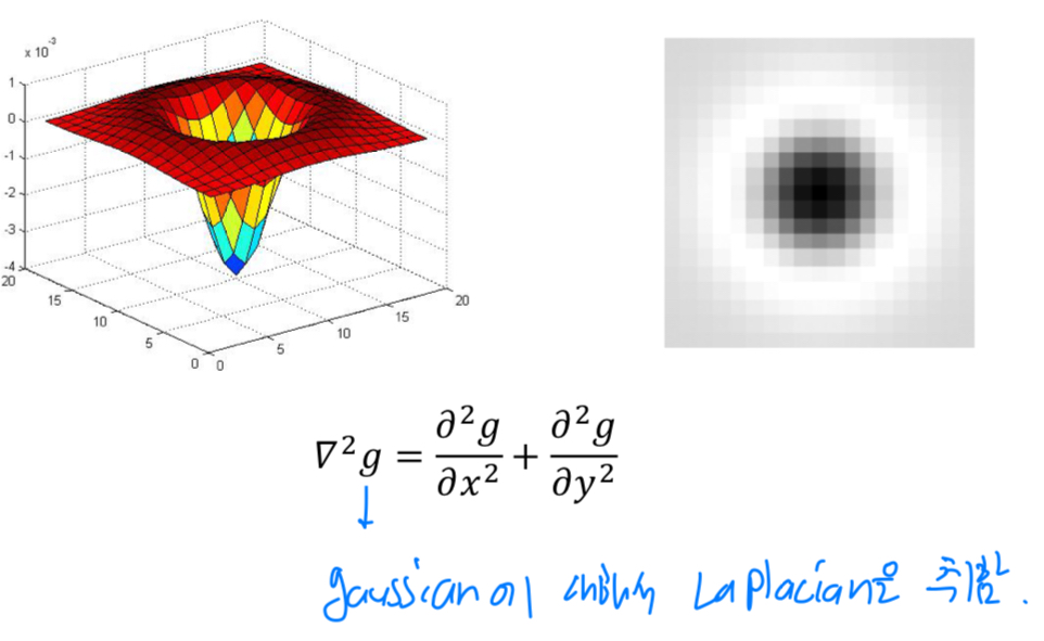
  이때 일반적으로 사용하는 kernel은 Laplacian of Gaussian(LoG) kernel이다.
  LoG는 Gaussian에 대한 함수를 2번 미분한 kernel이다.
  

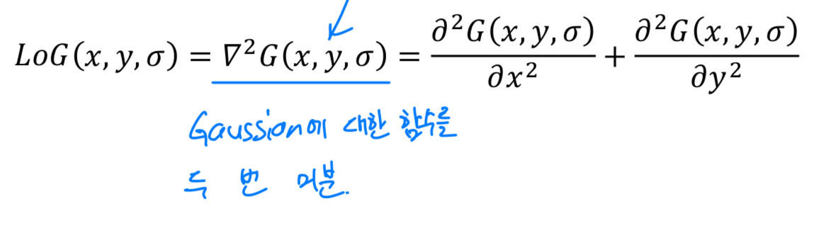
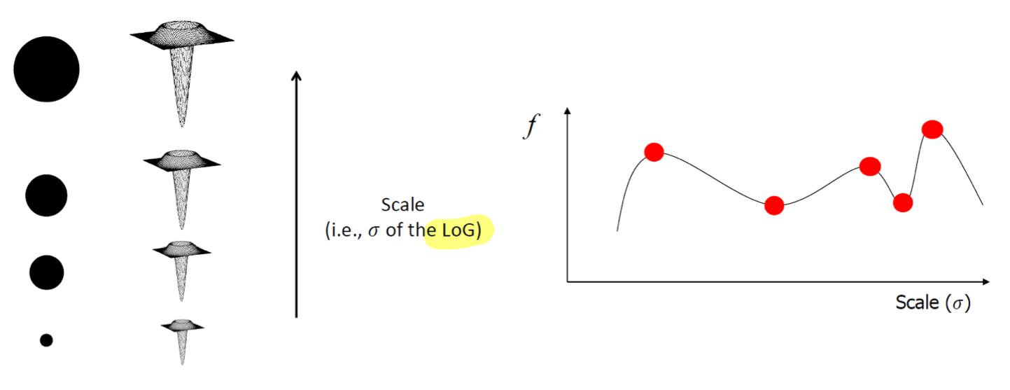
  Laplacian of Gaussian kernel을 사용하여 극값을 찾아내 원하는 scale을 찾아낼 수 있다.

Rotation invariant

• Rotation에 invariant한 descriptor를 찾아보자.

• Harris detector에서 eigen vector를 담고 있는 $M$ matrix가 존재했었는데,
  $M$으로 dominant한 방향을 찾는다면,
  해당 image가 어느정도 rotation되어있는지 알 수 있다.
  = image에 대한 principal axis를 찾는 것임
  
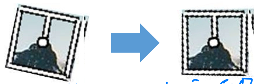
  찾은 후, warping을 통해 우리가 원하는 좌표계로 옮겨올 수 있다.
  이러한 과정은 gradient histogram을 이용해서 진행된다.
  
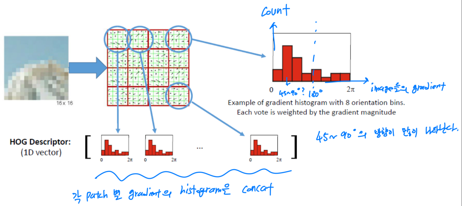
  HOG descriptor :
  각각의 image에 대해서 gradient를 계산하고,
  gradient에 대한 histogram을 생성.
  image의 특정 patch들에 대해서,
  각 patch들의 gradient가 향하는 방향을 bin을 x축으로 구성하고,
  그 count들을 y축으로 설정하면,
  해당 gradient들에 대한 histogram을 concat시켜 HOG descriptor를 만들게 되어,
  해당 image가 어떤 방향으로 orientation되었는지 알 수 있게 된다.

How to determine the patch orientation?

• patch의 orientation을 확인하는 방법
  1. image에 Gaussian kernel을 적용하여, blur한 image를 만듦. (전처리)
  2. gradient vector를 계산 (Harris detector M?)
  3. build a histogram of gradient orientations,
     this histogram is a particular case of HOG descriptor
  4. extract all local maxima in the histogram
  5. image warping

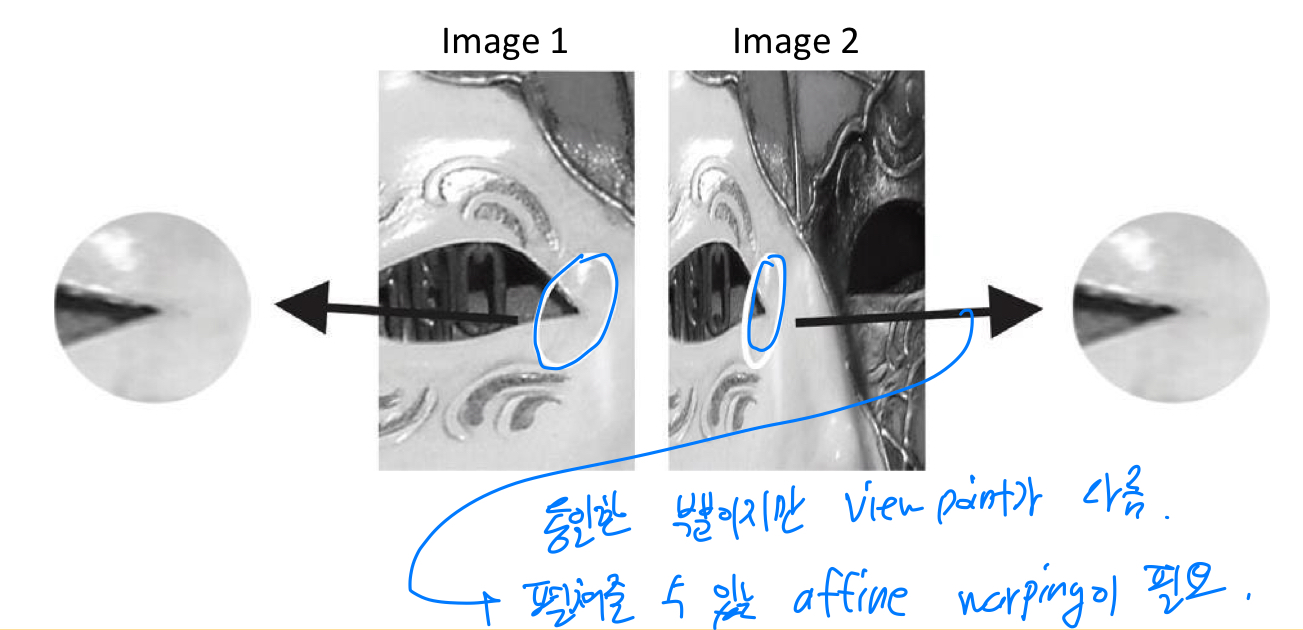
viewpoint invariant

• viewpoint에 따라 receptive field가 달라서, 찌그러진 image를 펼쳐줄 수 있는 affine warping이 필요하다.
  

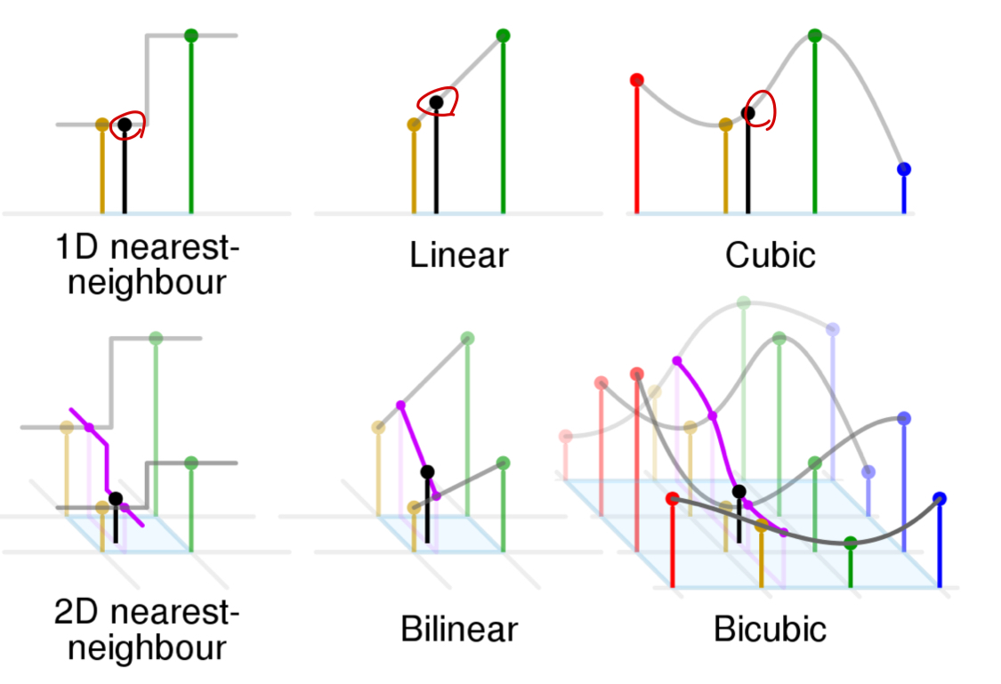
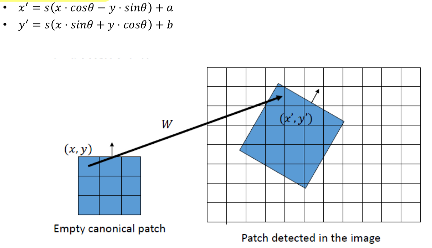
How to warp a patch?

• warping :
  warping하고자 하는 pixel과 인접한 pixel간의 관계를 이용해서 interpolation(보간)해준다.
  interpolation 방법은 다양하다.
  • Nearest neighbor interpolation
  • Bilinear interpolation
  • Bicubic interpolation
    
• warping function W :
  rotation($\theta$) + rescaling($s$) + translation($a, b$)이 모두 적용된다.
  

---

Blob detector

recall

• Harris detector :
  Harris detector는 matrix $M$의 eigen value를 이용하여 rotation invariance에 사용됐었음.
  하지만 scale non-invariance했었음.
  ➡️ corner detector로서 한계를 갖고 있다.

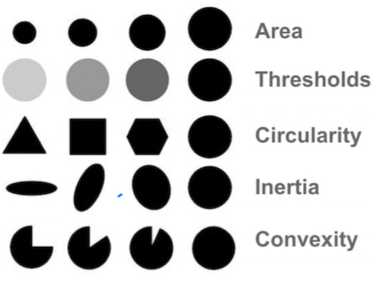
Blob detection

• Blob :
  Binary large object.
  image 내에 pixel들이 연결되어 있고, group을 나타냄.
  그 group이 공통적인 속성(밝기, 색상, 모양, 등)을 share하고 있음.
  

Blob filter

• Blob filter를 이용하여 Blob을 detection할 수 있음
  

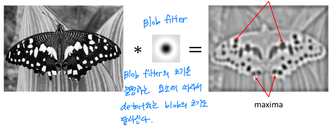
• Blob filter는 Laplacian of Gaussian(LoG = DoG 2번 적용)를 적용한다.
  

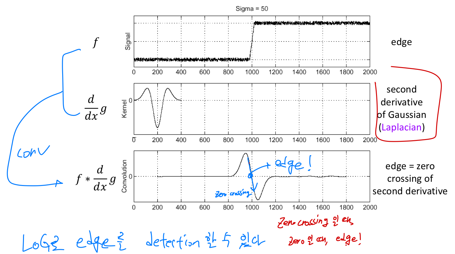
  • LoG로 edge를 detection했었음
    

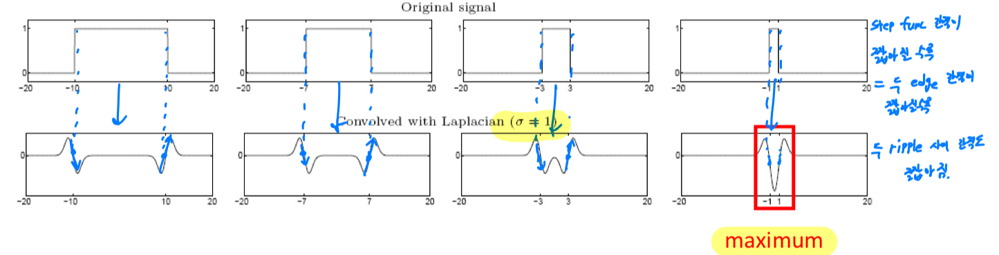
• From edge to blobs
  edge = ripple(잔잔한 물결)
  blob = 2개 ripple의 중첩
  으로 해석할 수 있다.
  LoG는 DoG에 의해 이루어지고,
  DoG에서 적절한 $\sigma$를 찾는 것이 blob에 대한 올바른 scale을 찾는 데에 중요한 요소가 된다.

Effect of Scale Normalization

• blob에 적합한 scale을 찾고 싶은데, 특정한 $\sigma$로 정해져있는 Lapacian kernel을 활용할 것이다.
  그 Laplacian kernel에 대한 maximum response를 찾을 것이다.
  하지만 문제가 발생한다.
  
  Laplacian에 대한 response는 scale이 커질수록 response가 작아진다.
  위에서는 $\sigma=1$로 고정된 상태로 signal의 길이만 늘려간 것이다.
  하지만 $\sigma$가 점점 커질수록 original signal에 대한 LoG response는 점점 작아지게 된다.
  

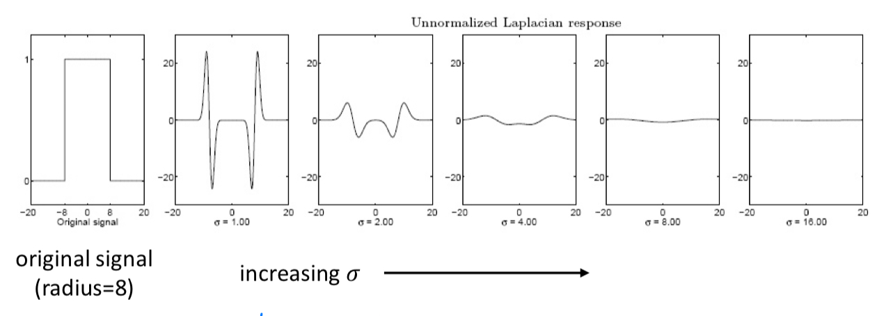
  우리는 response가 maximum, minimum이 되는 영역이 존재해야 해당 영역이 blob이라고 detection할 수 있었는데,
  Gaussian의 $\sigma$가 커질수록 해당 signal에 대해서 LoG를 적용했을 때, 그에 대한 response가 decay되어 blob을 detection하기 힘들어진다.
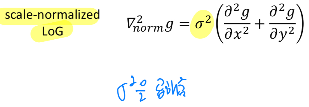
  따라서 Gaussian kernel에다가 scale factor를 곱해주는 형태로, LoG를 형성하게 된다.
  
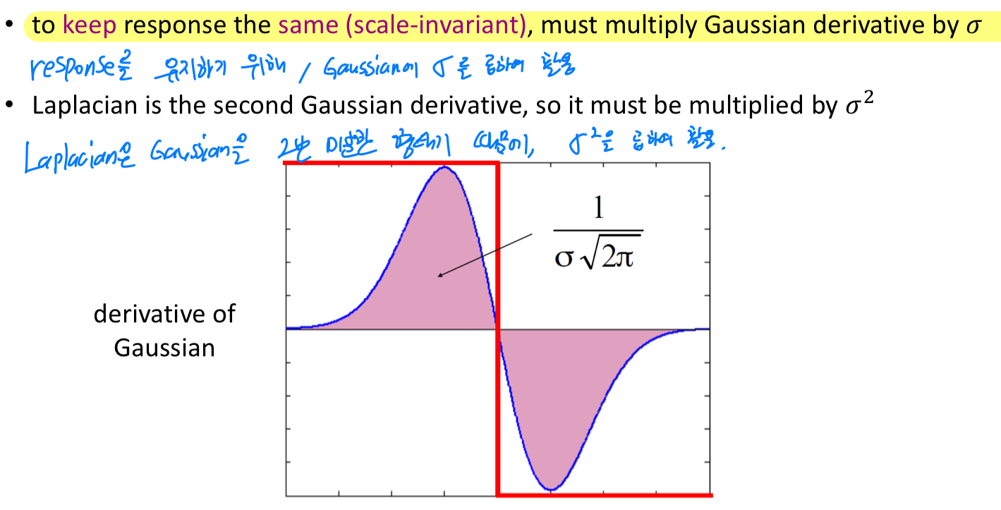
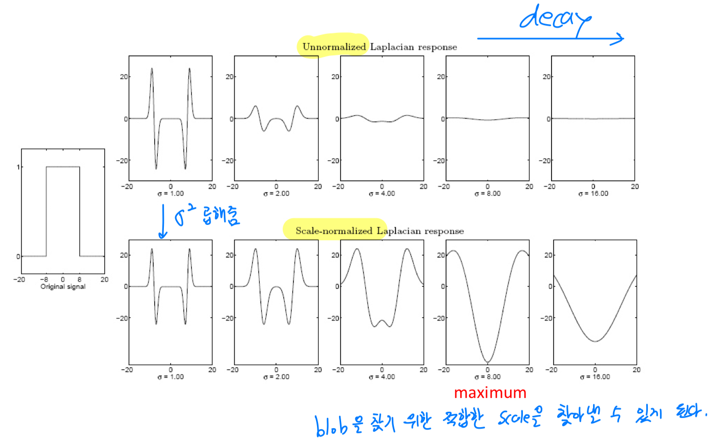
  따라서 scale-normalized LoG는 다음과 같다.
  

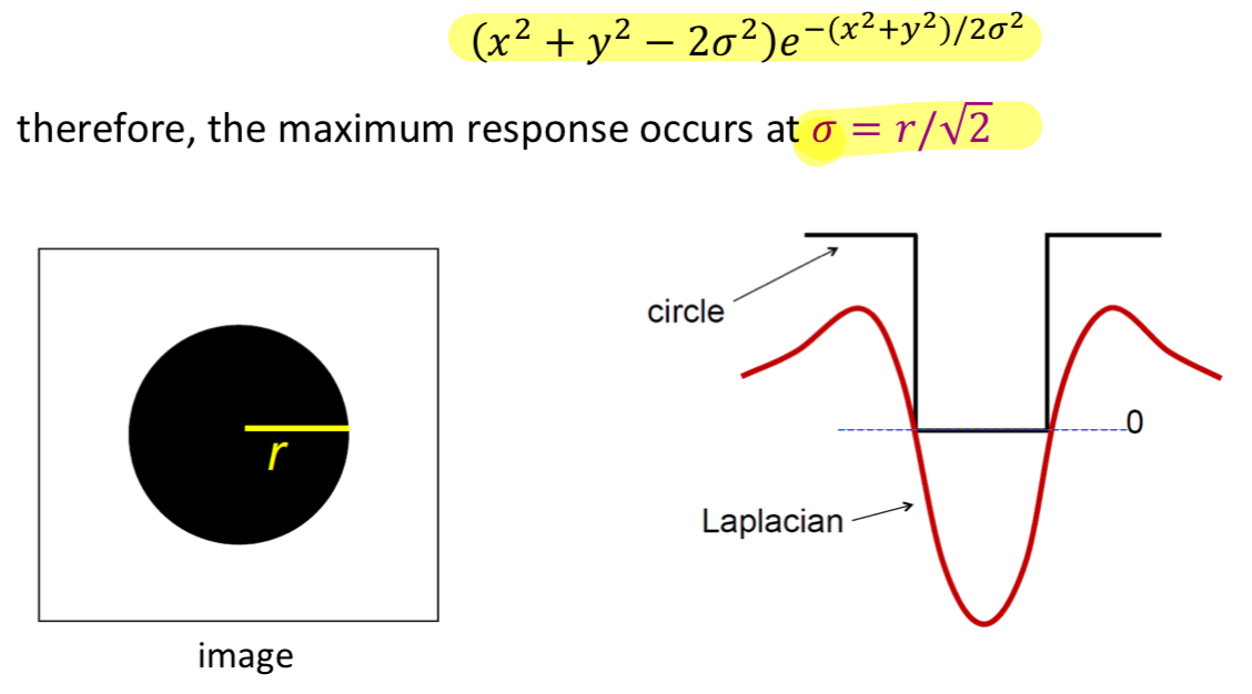
Scale selection

• 그러면, 이제 어떤 scale일 때 LoG이 maximum response를 보일까?
  ➡️ $\sigma$에 대해서 미분하고, 그것을 0으로 놓고, $\sigma$는 얼마인가? 를 찾으면 극값을 알 수 있다.
  그때의 극값 = $\sigma = r / \sqrt2$
  

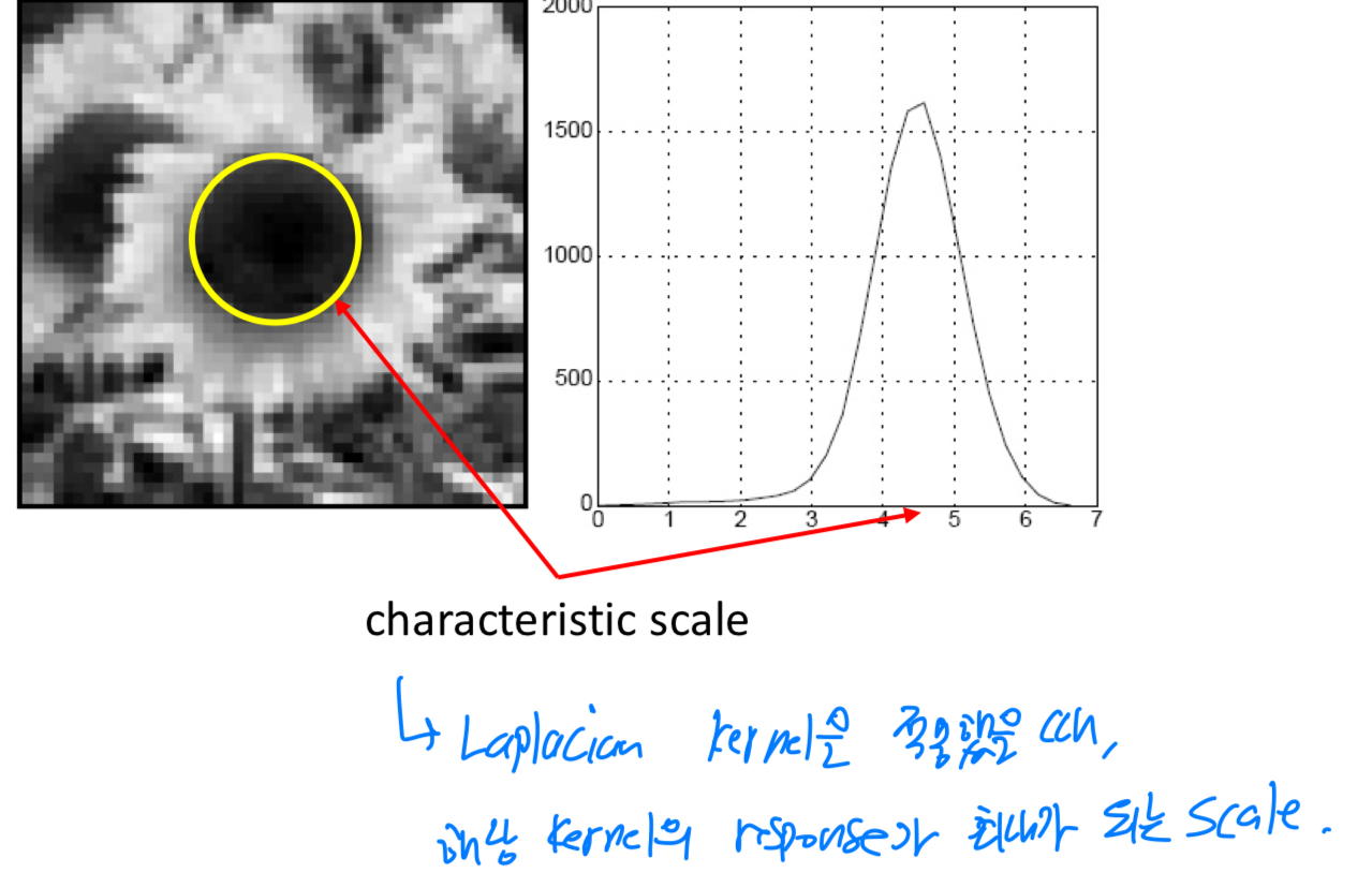
• characteristic scale :
  Lapacian kernel을 적용했을 때, maximum response를 보이는 scale값.
  

---

SIFT descriptor

• SIFT : Scale Invariant Feature Transform
  SIFT는 다음의 속성들에 대해서 invariant하다.
  • translation
  • rotation
  • scaling

SIFT keypoint computation

• SIFT의 computation은 크게 4가지로 이루어져 있다.
  1. scale-space extrema detection :
     Laplacian pyramid(=difference of Gaussian=DoG)를 활용해서
     모든 scale에 대한 극값을 찾아낸다.
  2. keypoint localization and filtering :
     image 내에서 특정 candidate들을 찾아내어, 불필요한 값들을 없앰.
  3. orientation assignment :
     해당 영역(keypoint)가 어떤 orientation(=gradient 방향)을 갖고 있는지 찾아냄
  4. creation of SIFT keypoint descriptor :
     keypoint descriptor를 만들어내는 과정.
     image를 matching시키기 위해 해당 image를 특정한 vector 형태로 바꾸는 과정이 필요함.
     그래서 주어진 image에서 특정 속성들을 뽑아낸 후, 수치화시키는 과정.

1. scale-space extrema detection

• Blob들을 찾아내기 위해서 characteristic scale을 확인했었는데,
  이러한 것들을 찾아내기 위해서 어떻게 scale-space를 표현하는가?
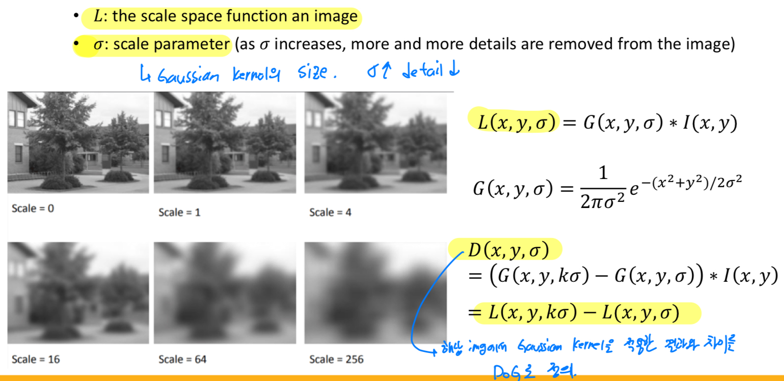
  ➡️ 원본 image에서 점진적으로 blur한 image를 만들어 낸다.
  image에 대해서 Daussian filter를 적용하여 blur하게 만든다.
  ➡️ 이때, $L$로 표현되는 scale space function이 정의된다.
  주어진 image에서 Gaussian kernel을 적용한 결과와 차이를 DoG로 정의.
  

• 그런데 LoG를 계산할 때, Gaussian kernel size가 커짐에 따라서 LoG에 대한 response가 decay되는 것을 확인했었음.
  따라서 scaled-normalized LoG를 적용.
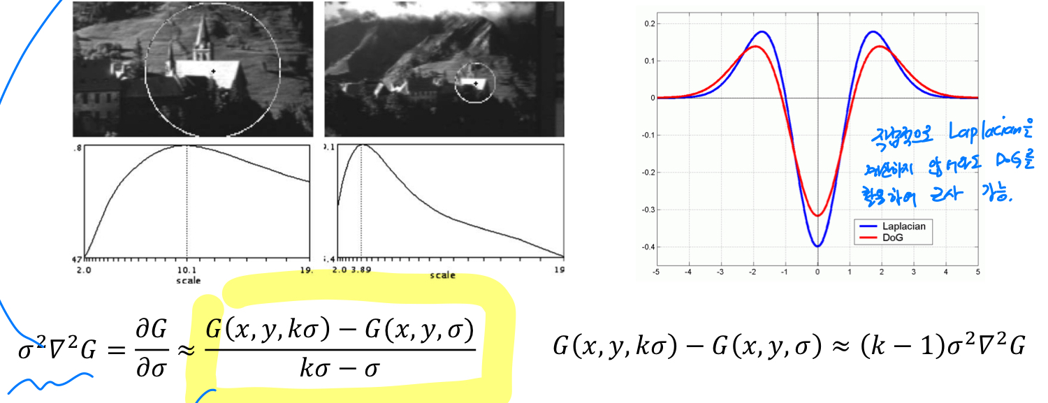
  하지만, LoG를 계산하기 위해 x, y에 대한 2차 편미분을 계산해야 하기 때문에 computational cost가 크다.
  특정 연구에서, DoG 함수의 차이로 근사할 수 있다고 확인되어졌다.
  따라서 직접적으로 LoG를 계산하지 않고, DoG 함수의 차이를 이용하여 LoG를 근사할 수 있다.
  

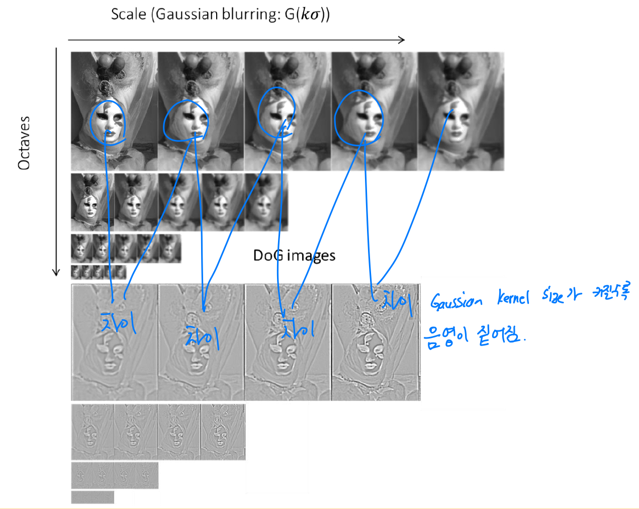
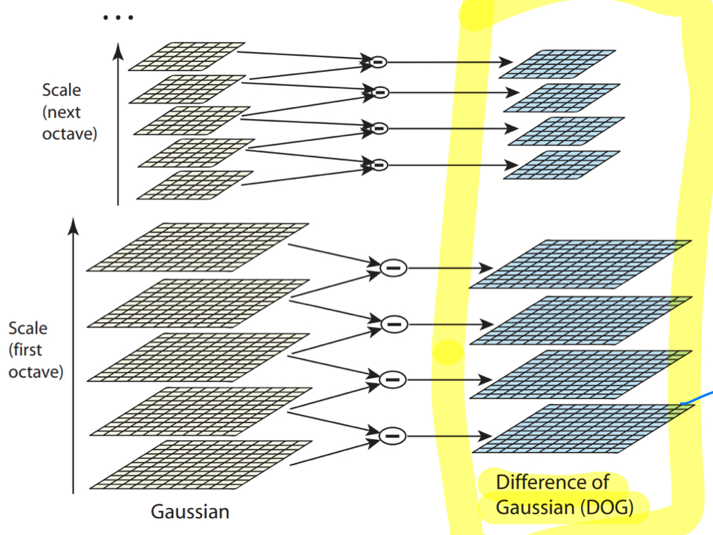
• 그래서 Gaussian kernel size를 점진적으로 크게하여 점진적으로 blur되어진 image들에 대해서
  DoG를 계산한다.
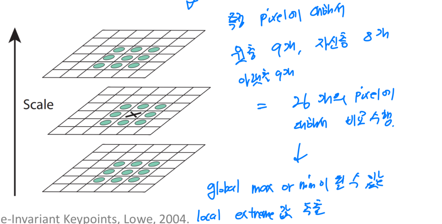
  이때, 가운데 있는 층(3x3)과 위아래 층들을 비교하여
  global max or min이 될 수 있는 local max or min를 추출하여,
  SIFT keypoint의 candidate로 갖게 된다.
  

2. keypoint localization and filtering

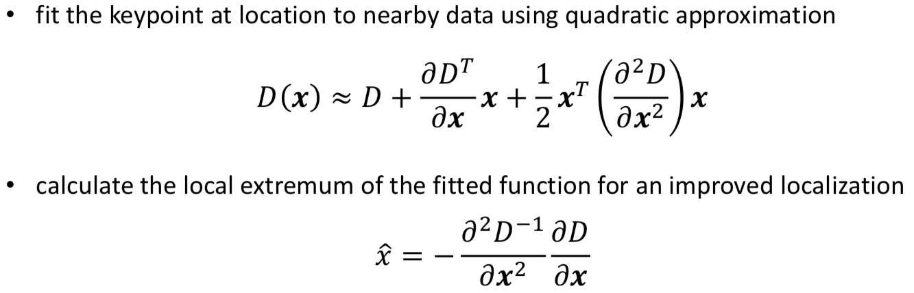
• 실제 극값이 아닌데 candidate된 값들이 존재하므로, 그 점들에 대해서 정제하기 위해 2차 근사를 하여 지운다.
  

• 추가적으로 후처리가 또 필요하다.
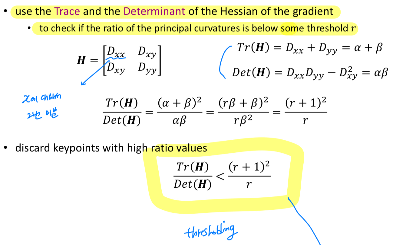
  corner 근처에서 2가지 이상의 gradient를 갖게 될 수 있다.
  따라서 방향성을 고려한 filtering 과정이 필요하다.
  Harris detector에서처럼 hessian을 정의하여, trace와 det를 적용하여 thresholding을 적용한다.
  

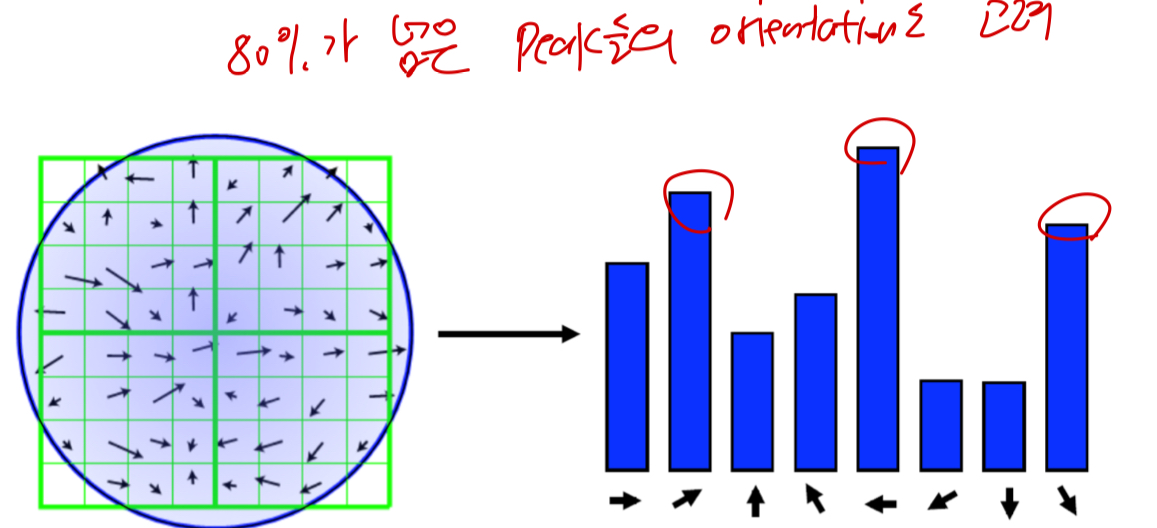
3. orientation assignment

• 우리는 rotation과 scale에 invariant한 keypoint들을 찾고 싶기 때문에
  descriptor를 통해서 해당 point(feature)가 갖고 있는 rotation과 scale에 대한 정보를 encode하고 싶다.
  
  이를 위해서 gradient의 magnitude와 orientation을 계산한다.
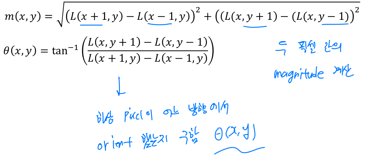  그리고나서,
  각각의 orientation에 대해서 histogram of local gradient(HOG descriptor)를 구한다.
  80%가 넘는 peak들에 대한 orientation들 모두 고려.
  

4. creation of SIFT keypoint descriptor

• 지금까지 SIFT keypoint descriptor가 되기 위한 candidate를 만들어왔고, 정제하는 작업을 거쳤다.

• 우리가 갖고 있는 정보 : image 좌표(x, y), scale 정보($\sigma$), magnitude(m), orientation($\theta$)
  를 이용하여 illumination과 viewpoint에 invariant한 local descriptor를 만들어 낼 것이다.

• 4x4=16개의 patch에 대해서 Gaussian kernel를 적용하여 noise를 제거하고,
  각각의 Patch에 대해서 histogram을 계산하여 8가지 방향에 대해 계산된 orientation 정보로
  총 4 x 4 x 8 = 128 차원의 feature vector를 추출한다.
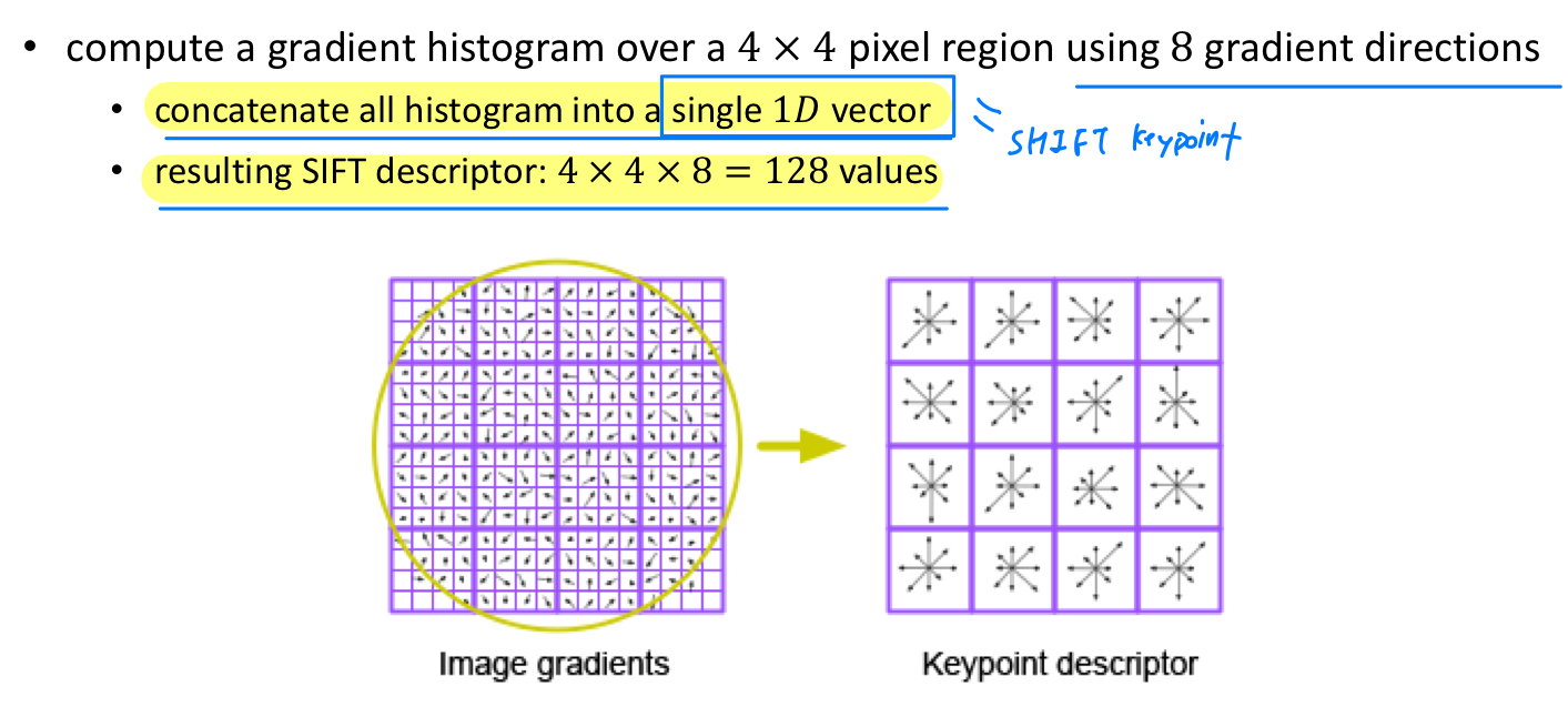  만들어진 128차원의 descriptor vector를 illumination에 invariant하도록, L2 normalization을 적용.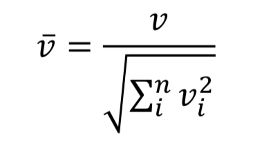최종적으로 만들어진 SIFT feature들은 viewpoint에 대한 강인한 속성을 보인다.
  최대 50 degree rotation에도 robust함.
  또한 illumination의 변화에도 robust함.
  
  하지만, computational resource가 많이 필요하다는 단점이 있다.

• repeatability도 좋기 때문에 matching에 좋은 algorithm이라고 볼 수 있다.

• 4x4 patch에서 성능이 saturation되기 때문에, 일반적으로 각 descriptor에 대해서 width를 4로 한다.
  또한 orientation을 8개로 나누는 것이 일반적이다.
  

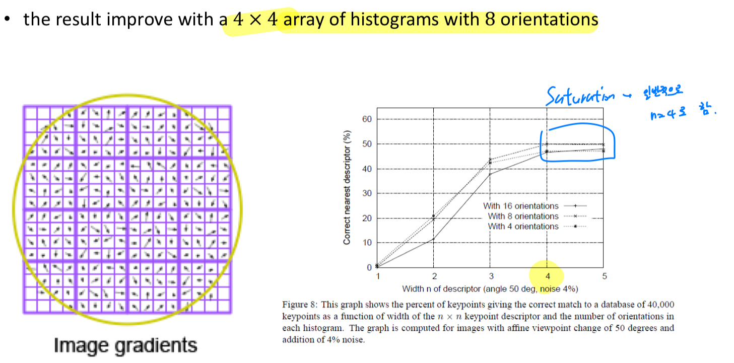
• object recognition, panorama stitching에 사용된다.