Introduction to Segmentation and Clustering

• Segmentation :

  • identify groups of pixels that go together
  • separate image into coherent(동등한) "objects"

• Major process for segmentation :
  token = segmentation을 수행하기 위한 작은 unit.

  1. bottom-up :
     고전적인 algorithm.
     group tokens with similar features
  2. top-down :
     최근 Deep Learning의 기반한 방식들.
     커다란 part를 조각난 part들로.

• clustering :

  • 어떠한 유사성에 의해서 data를 묶어나가는 작업.
  • unsupervised learning method이다.
  • 어려운 점 : 어떤 point들이 유사한가? 몇 개의 group으로 묶을 것인가?

How do we cluster?

1. agglomerative clustering :
   tree형식으로 각각의 cluster가 자기 자신의 cluster를 찾아나감
2. k-means :
   가장 보편적으로 사용되는 clustering 방법.
   k = #clusters
3. mean-shift clustering :
   평균을 이동시켜서 clustering

1. Agglomerative Clustering

• Agglomerative Clustering = bottom-up hierarchical clustering

• Algorithm :

  • initialization :
    각각의 point들을 own cluster로 생성.
  • repeat :
    N개의 쌍이 있다면, N개의 쌍 각각의 거리를 계산
    그 중에서 가장 유사한 pair를 찾으며 묶어나감.
  • until :
    그 작업을 우리가 원하는 cluster수에 도달할 때까지 수행.
    또는
    only one cluster가 될 때까지 수행.

• clustering의 결과를 Dendrogram(tree)으로 나타낼 수 있다.
  

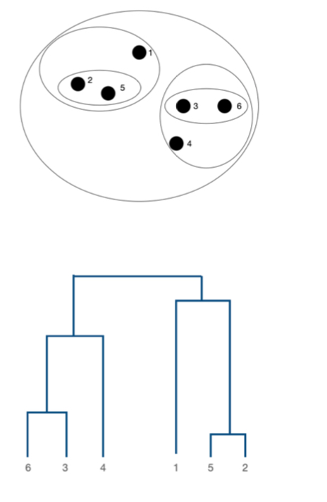
• Agglomerative Clustering에서 heuristic하게 적용되는 method :
  How to define cluster similarity?
  정답은 없고, 해봐야 안다.

  • minimum distance
  • maximum distance
  • average distance between points

• 장점 :

  • 간단하다
  • adaptive shapes (shape이 갑자기 확 생기지 않음)

• 단점 :

  • imbalanced cluster
  • $O(n^2)$ time complexity

2. K-means Clustering

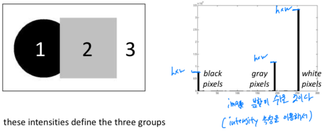
• 간단한 image가 있을 때, 우리는 pixel의 intensity로 clustering을 쉽게 수행할 수 있을 것이다.
  하지만 Gaussian noise가 있다면? 다음과 같을 것인데,
  intensity가 겹치는 부분에 대해서 어떻게 clustering을 할 것인지? 애매한 점이 있다.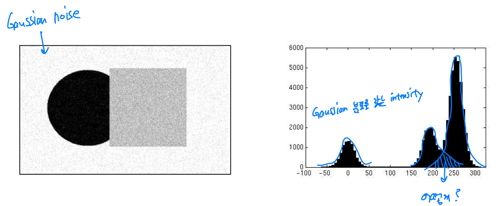

• 그래서 우리가 가지고 있던 intensity feature를 1차원으로 mapping시키면 다음과 같은데,
  가운데에 애매하게 위치하여 있는 feature들을 어느 center(C)로 줄 것인지를 결정해야 한다.
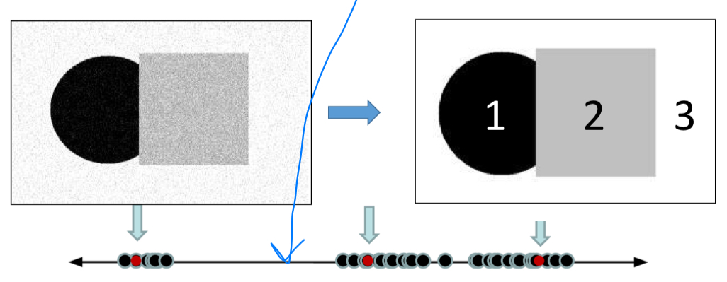  각각의 cluster에 대해서는 center(C)가 존재하고,
  data들과의 거리 SSD(sum of square distance)를 계산하여,
  Center와 data들 간의 SSD가 가장 작은 곳을 Center로 정한다.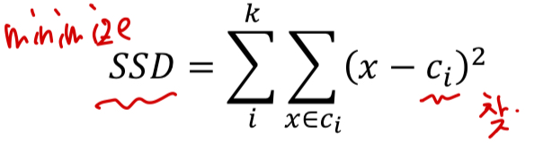이러한 원리가 K-means에 그대로 적용된다.

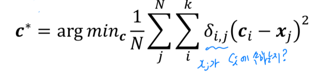
• goal, object function :
  $N$개의 주어진 data가 있을 때, $k$개의 cluster로 할당시켜야 한다.
  그래서 center와 data 사이의 거리(=SSD)를 minimization하는 방향으로 학습하여
  center(C)와 $\delta$를 찾는 것이 목적.
  ($\delta_{i,j}$ : $c_i$와 $x_j$를 이을 것인지 판단하는 binary value. = mask)
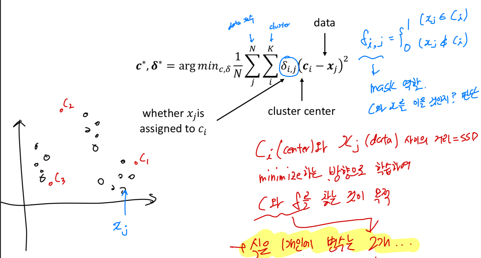  우리의 목적을 만족시키는 식은 1개이지만, 찾아야 하는 변수는 2개이다.
  따라서 iterative하게 optimum을 찾아야 한다.

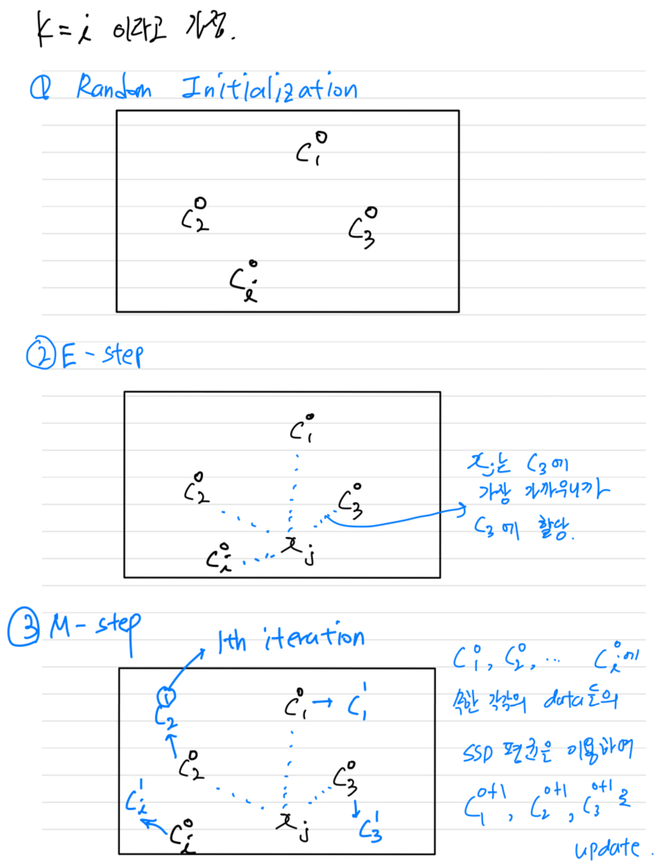
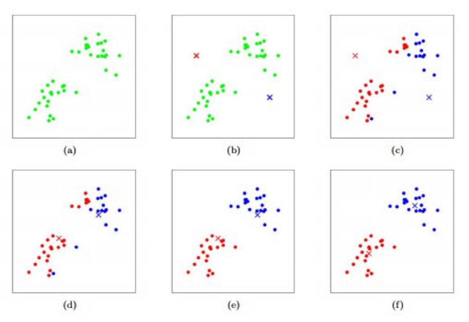
K-means clustering algorithm

1. initialization :
   우선 $k$개의 center $c$를 random하게 initialization
   

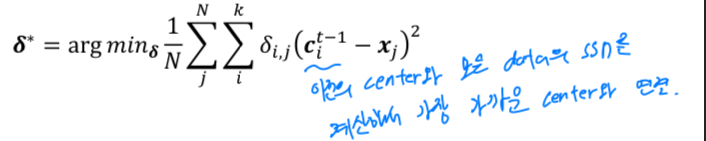
2. E-step (assignment step) :
   각 cluster의 center(c)와 data의 SSD를 비교하여, 가장 가까운 cluster의 center(c)에 할당해주는 과정 = data에 label을 할당해주는 과정
   
   

3. M-step (update step) :
   각 cluster의 center(c)와 그 cluster에 속하는 data들의 SSD 평균을 사용하여 center(c)를 update.
   

4. termination : E, M step을 반복적으로 수행.

   • iteration이 정해진 maximum number에 도달하거나,
   • 더 이상 assignment가 변하지 않을 때까지
     

     k-means는 Local optimum을 찾는 것이다.
     global optimum을 찾을 수 있겠지만 조건이 매우 까다롭다.
     (초기화에 따른 영향이 많이 있다. extremely sensitive.)
     

how to initialize?

• 초기화는 일반적으로 random하게 초기화한다.
• k-means++에서는 center들을 최대한 넓게 퍼져있도록("spread-out") 초기화

how to choose K?

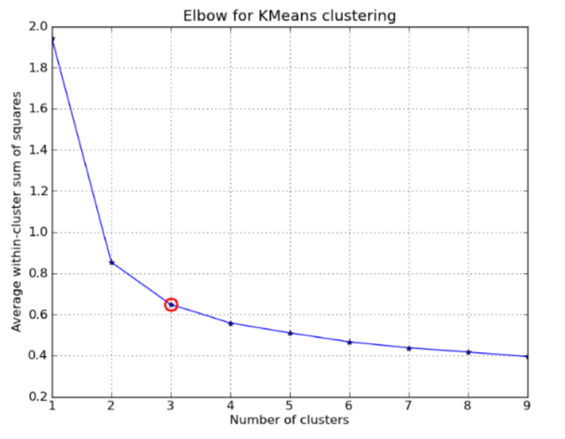
• elbow point :
  몇 개의 cluster가 최적인지 알 수 없다.
  따라서 최적의 K를 결정하기 위해서는 모든 K를 해볼 수 밖에 없다.
  각 K 별로 SSD를 계산하여 graph로 시각화해보면,
  'elbow point'가 나타난다.
  여기서는 cluster가 3인 부분에서 어느정도 SSD가 saturation된다.
  너무 많은 cluster로 나누면, 똑같은 class를 너무 세분화하여 나눠질 수 있기 떄문에 좋지 않다.
  

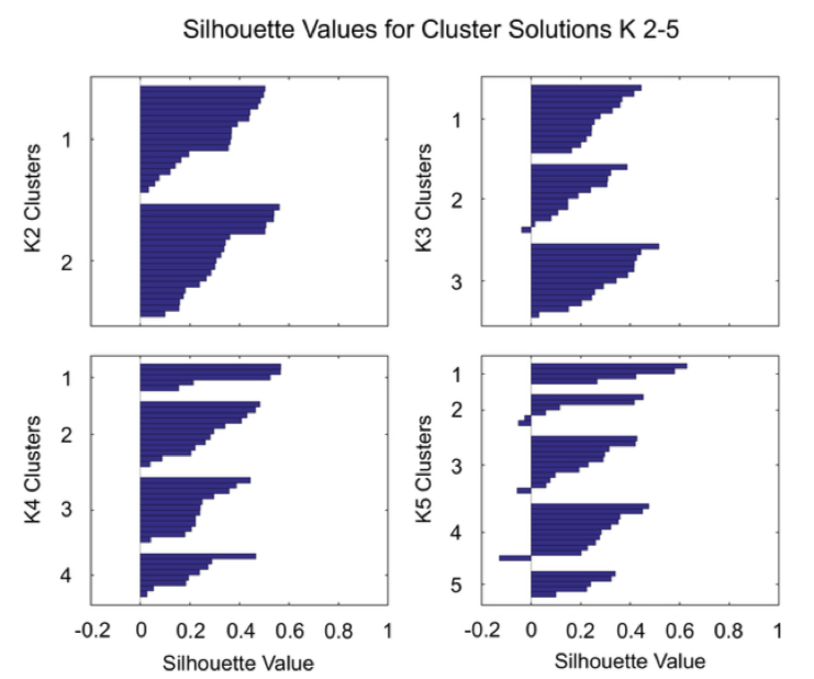
• silhouette value (실루엣) :
  center쪽으로 data들이 뭉치는 속성과
  cluster들끼 서로 멀어야 하는 속성이 있어야 좋은 cluster이다.
  이러한 속성을 나타내는 지표.
  
  graph가 빵빵하게 많이 차있는 것을 좋은 것으로 봄.
  

• validation set

distance measure & termination

• distance measure :
  • Euclidean (commonly used)
  • Cosine
  • non-linear (kernel method)
• termination :
  • 미리 정해놓은 maximum number iteration에 도달했을 때, 종료
  • assignment step에서 변화가 없을 때, 종료

Segmentation as clustering

• 단순히 intensity만으로 clustering할 수도 있고,
  color similiarity로 clustering할 수도 있다.

• 하지만 color로만 RGB image를 의미 있는 class로 segmentation할 수 없다.

• 이를 막기 위해 texture similarity를 고려한 clustering을 고려할 수도 있다.

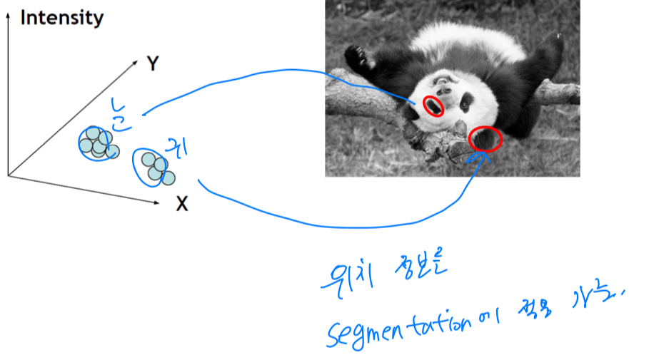
• 또한 intensity + position similarity도 고려하여 clustering할 수 있다.
  눈과 귀를 분류하기 어려운데, position 정보가 있다면 분류할 수 있다.
  

k-means limitations

1. hard assignment :
   1 or 0으로 극단적인 cluster 선택.

2. outlier example에 취약하다.

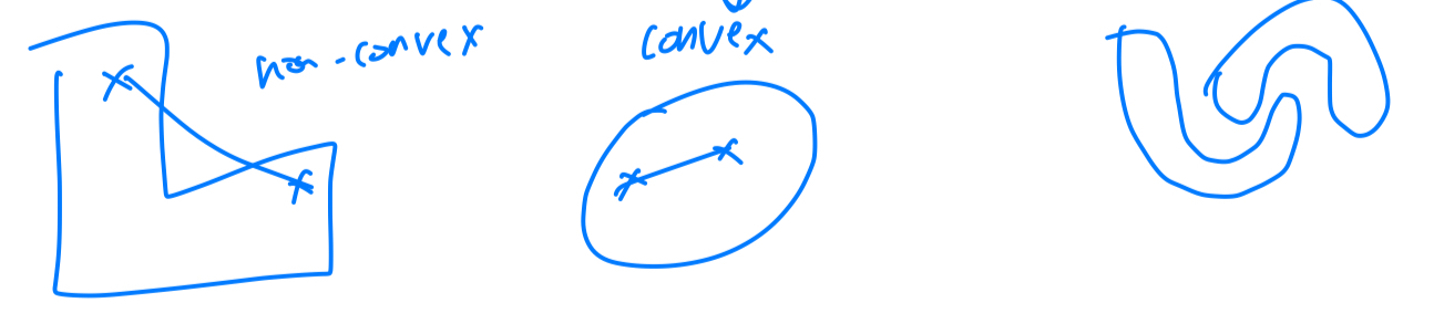
3. round shape에 대해서는 잘 작동하지만, non-convex shape에 대해서는 잘 동작하지 않는다.
   

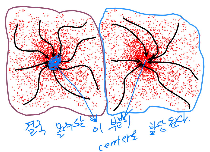
3. Mean-shift Clustering

• assumption :
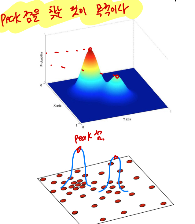
  주어진 data들이 확률 밀도 함수(probability density function, pdf)에 존재한다는 가정.
  data들을 확률 밀도 함수로 나타내었을 때, peak점을 찾는 것이 목적이다.
  

• Mean-shift :

  • Region of Interest(RoI)을 random하게 설정
    관심영역(RoI)의 중심과 이 안에 속하는 data들의 무게중심(Center of mass)이 일치하지 않을 것이다.
  • Center of mass 계산
  • RoI를 center of mass로 옮김. 이떄, vector를 mean-shift vector라고 함
    
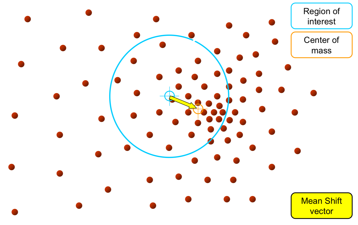
    이렇게 점차점차 data의 밀도가 높은 곳으로 옮겨짐.
    mean-shift vector가 0이 될 때까지 반복하여 수행.

• Mean-shift algorithm은 cluster의 개수를 설정 안해도 된다.

attraction basin

• data들이 몰려드는 이 부분이 center로 할당 되는데, 그 부분을 attraction basin(분지) 라고 함.