Logistic Regression

• Logistic Regression :
  예측하는 값을 확률적으로 접근
  Classification 장점 + Regression 장점

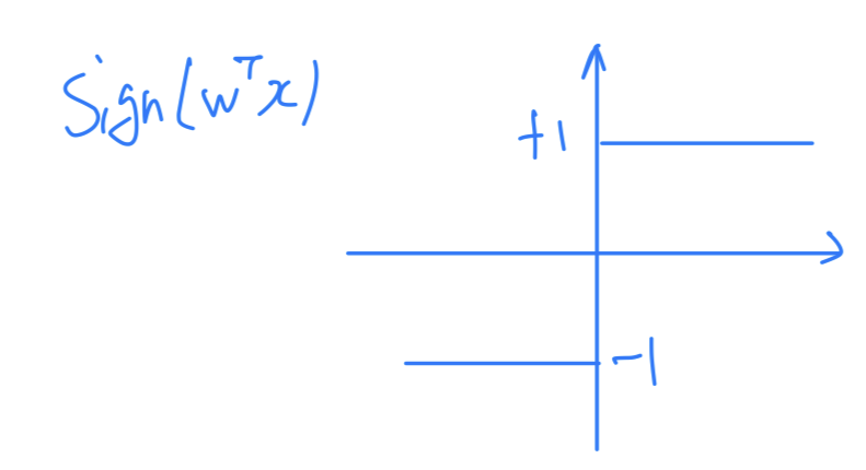
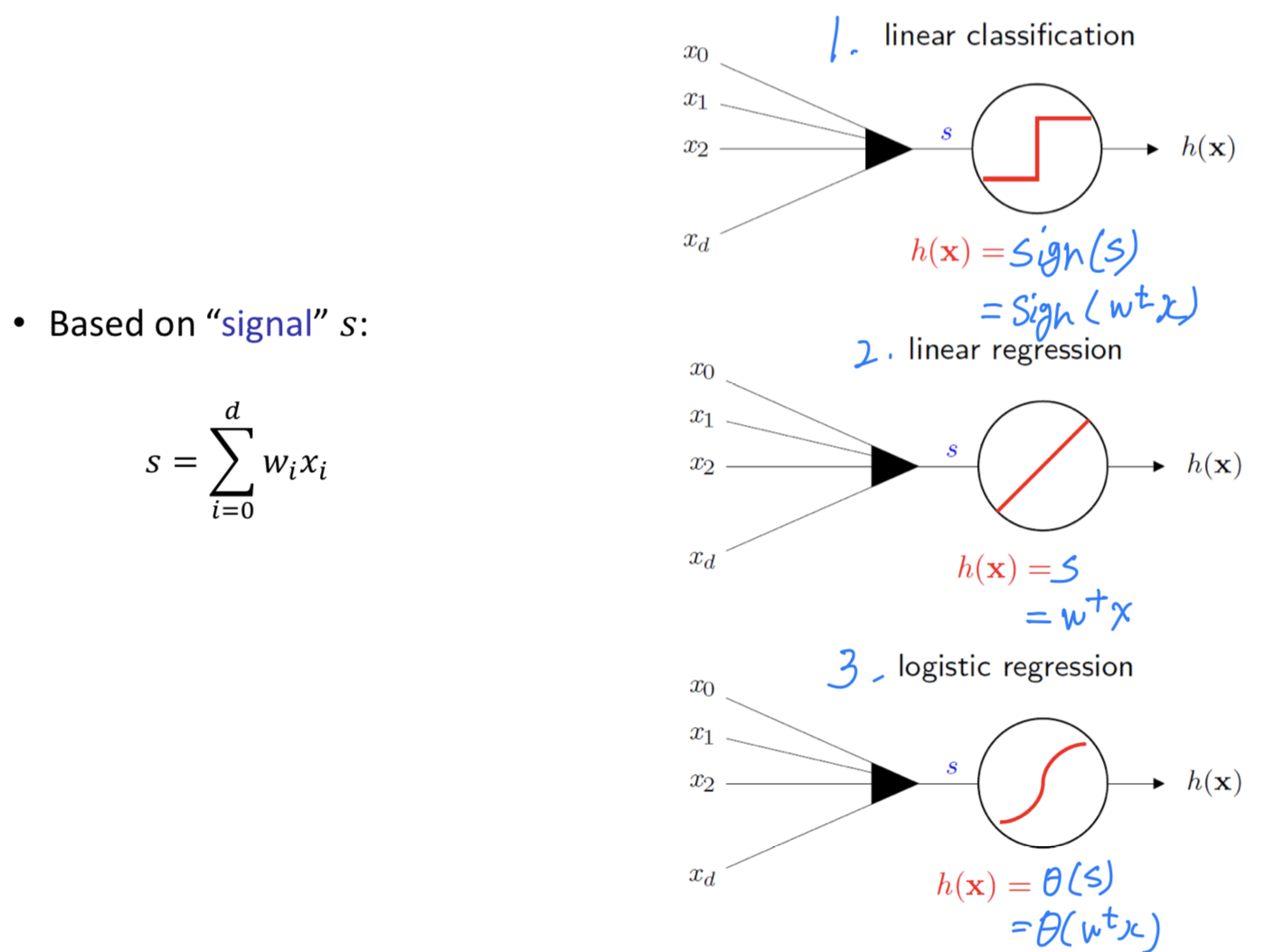
• Linear Classification
  : Signal is thresholded at zero to produce +-1 output
  For binary decisions
  ➡️ $sign(w^Tx)$
  

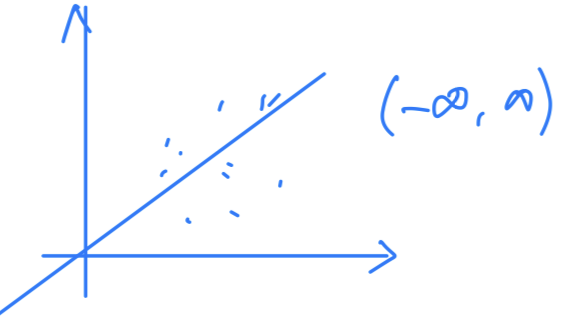
• Linear Regression
  : Signal itself = output
  For predicting real(unbounded) response
  ➡️ $w^Tx$
  

Motivating Example

• Heart Attack Prediction based on cholesterol level, blood pressure, age, weight, ...

• Cannot predict a heart attack with any certainty

• Linear Classification에서는
  심장마비가 "0.8만큼 일어났다" 는 없고,
  심장마비가 "일어났다(1)?" 또는 "일어나지 않았다(0)?"로만 관찰하게 된다.
  하지만 Logistic Regression은 심장마비가 얼마나 일어날 것인지([0, 1])를 예측할 수 있다.
  즉, hard classification이 아니라 soft label(probability)을 갖는다.

Logistic Regression : soft binary classification

• heart attack or not, dead or alive ➡️ Linear Classification
  Returns soft labels(probability) ➡️ Logistic Regression

• Output : real(like regression) but bounded(like classification)

• Comparison : Linear Regression vs Logistic Regression

  • Both deal with a binary event
  • Logistic Regression : allowed to be uncertain (불확정성에 대해 설명할 수 있다)

probability of default

• probability of default : 어떤 사람이 채무 불이행을 했냐? 안했냐?에 대한 확률

• 두 개의 class를 분류하기 위해서는 구분이 잘 되는 feature를 사용하여 구분해야 한다.
  

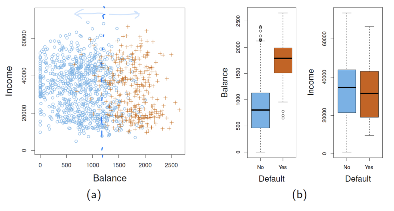
  • 위 예제에서는
    Balance(통장잔고)라는 feature를 사용해야 분류가 잘 될 것이다.
    ➡️ 특정 사람의 Balance가 주어졌을 때, 그 사람이 채무불이행을 했을 확률

• P[defualt = yes|balance] : probability of default given balance
  특정 사람의 Balance 정보가 주어졌을 때, 그 사람이 채무 불이행을 했을 확률을 구해보자.
  

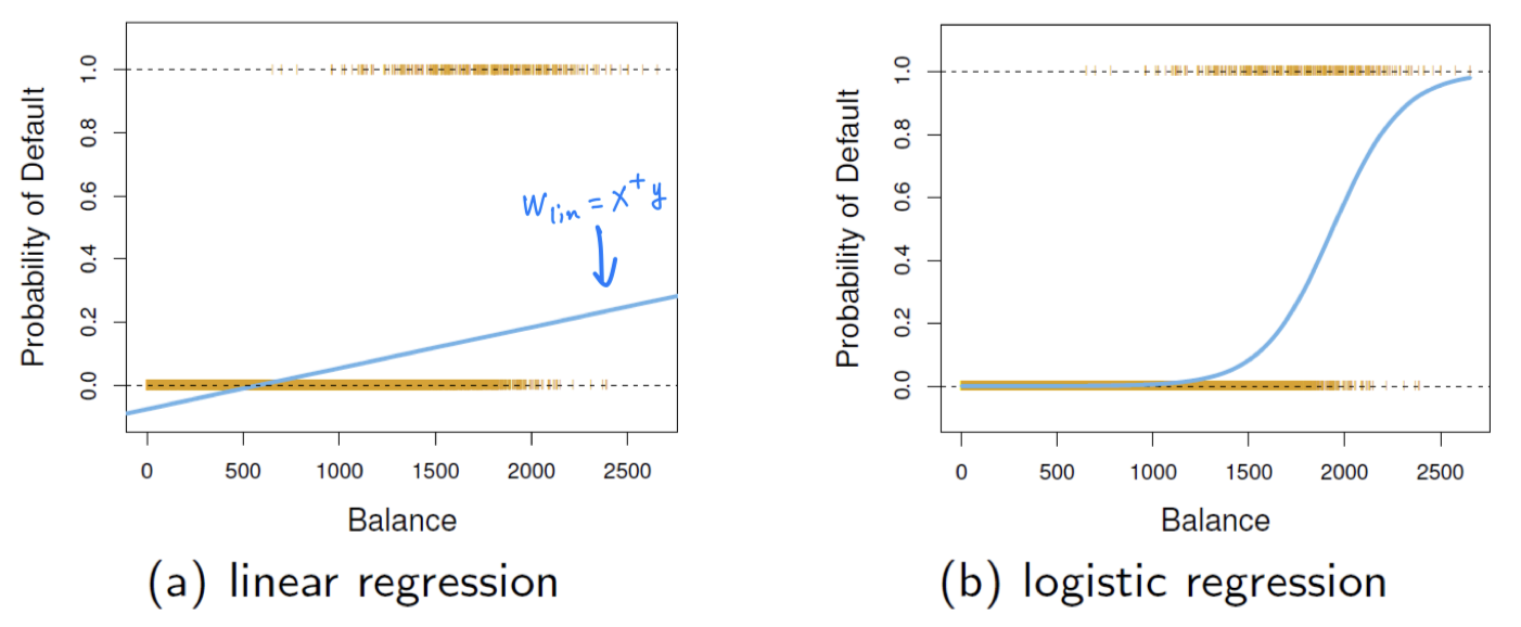
  • (a) : 직선은 음수의 값을 갖게 되는데, 확률은 음수를 가질 수 없기 때문에
    P[default = yes|balance]라는 Task에 부적합해보인다.
  • (b) : 우리가 원하는 0~1의 확률값을 가지면서 정확한 예측을 할 수 있다.

Linear model

1. Linear Classification : Hard Threshold on $signal$ $x = w^Tx$
   $h(x) = sign(w^Tx)$

2. Linear Regression : No Threshold
   $h(x) = w^Tx$

3. Logistic Regression : Output to probability range [0, 1]
   $h(x) = \theta(w^Tx)$, $\theta$ called logistic function == sigmoid function
   

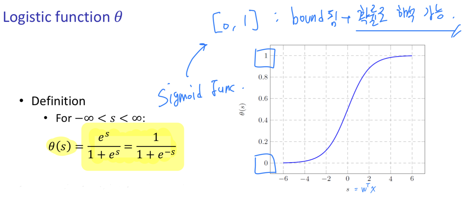
Logistic Function $\theta$

• Sigmoid Function == Soft Threshold
• Output lies between 0 and 1
  

Example : Heart Attack

• Prediction of heart attacks

  • Input $x$ : cholesterol level, age, weight, etc, ....
  • Signal $s = w^Tx$ : "risk score"
    
    
  1. Linear Classification
     ➡️ $h(x)$ returns +-1 : heart attack(+1) or not(-1)
  2. Linear Regression
     ➡️ $h(x)$ returns risk scores itself
  3. Logistic Regression
     ➡️ $h(x)$ returns $\theta(s)$ : probability of heart attack
     
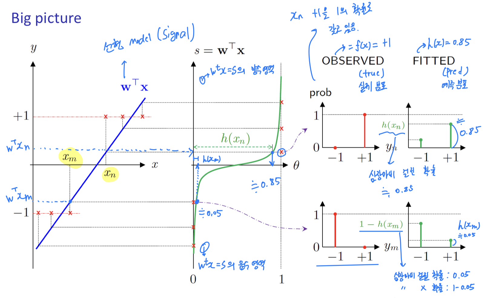
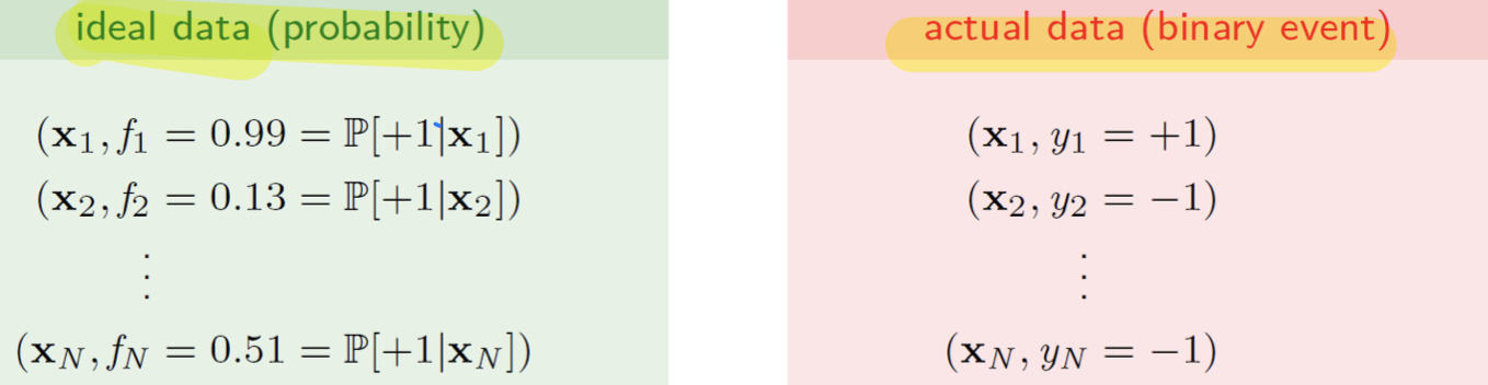
  • actual data는 "심장마비가 일어났다(+1)" 또는 "일어나지 않았다(-1)"라는
    binary event로 주어진다.
  • 우리는 그러한 예측을 잘 하기 위해서 Probability을 내뱉는 ideal data(model) 을 활용하는 것.

Cross-Entropy Error Measure

• We will use cross-entropy error measure
  

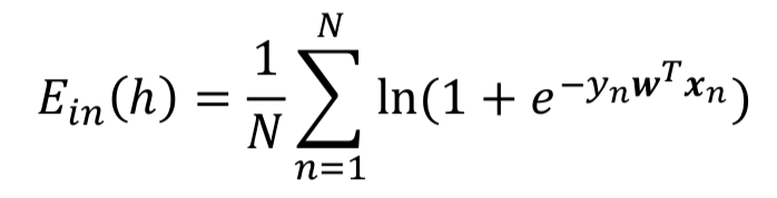
  1. Based on intuitive probabilistic interpretation (확률적 수행 가능)
  2. Has nice property for gradient-based optimization (기울기 최적화에 좋음)

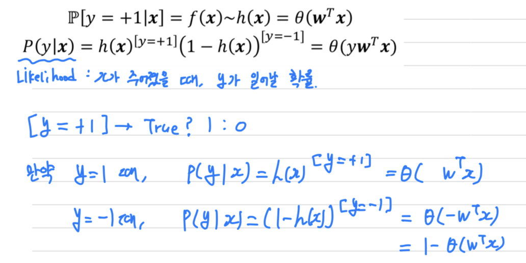
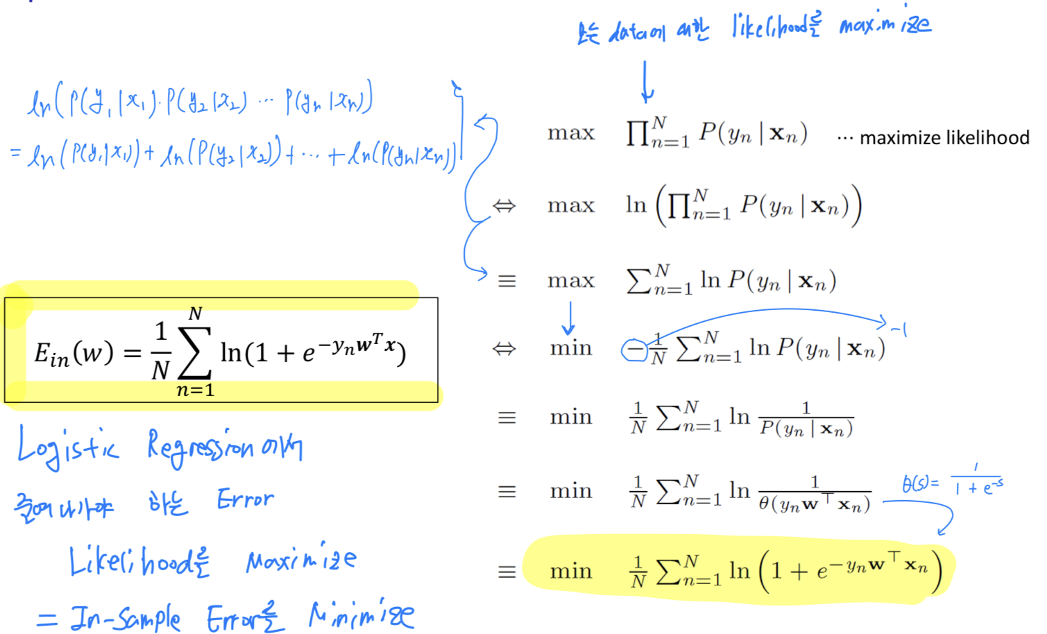
• Standard error measure in logistic regression : based on likelihood
  
  ➡️ data 하나하나마다 likelihood 정의.
  N개 data가 있으니까, N개의 Likelihood 정의

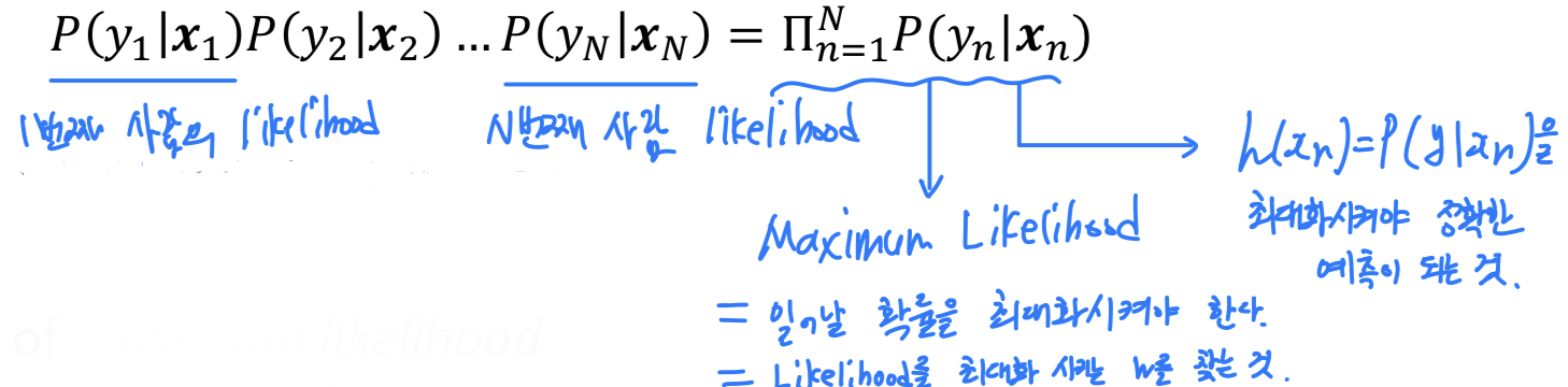
Criterion for choosing h : maximum likelihood

• 주어진 data를 모두 올바르게 분류하는 Probability를 계산해볼 것이다.

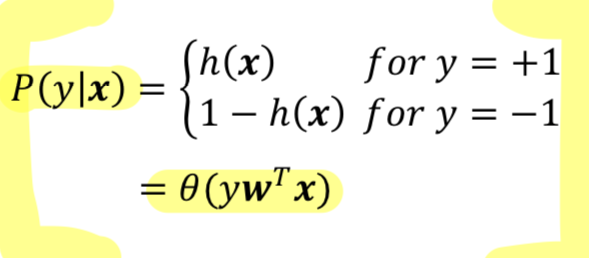
• N명이라는 사람이 있다고 가정하면, 각 사람에 대한 Likelihood는 다음과 같다.
  

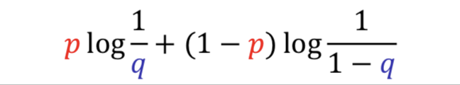
• Consider two pmfs $(p, 1-p)$, $(q, 1-q)$ with binary outcomes
  Cross entropy for these two pmfs : defined by
  $plog\frac{1}{q} + (1-p)log\frac{1}{1-q}$

• Let.
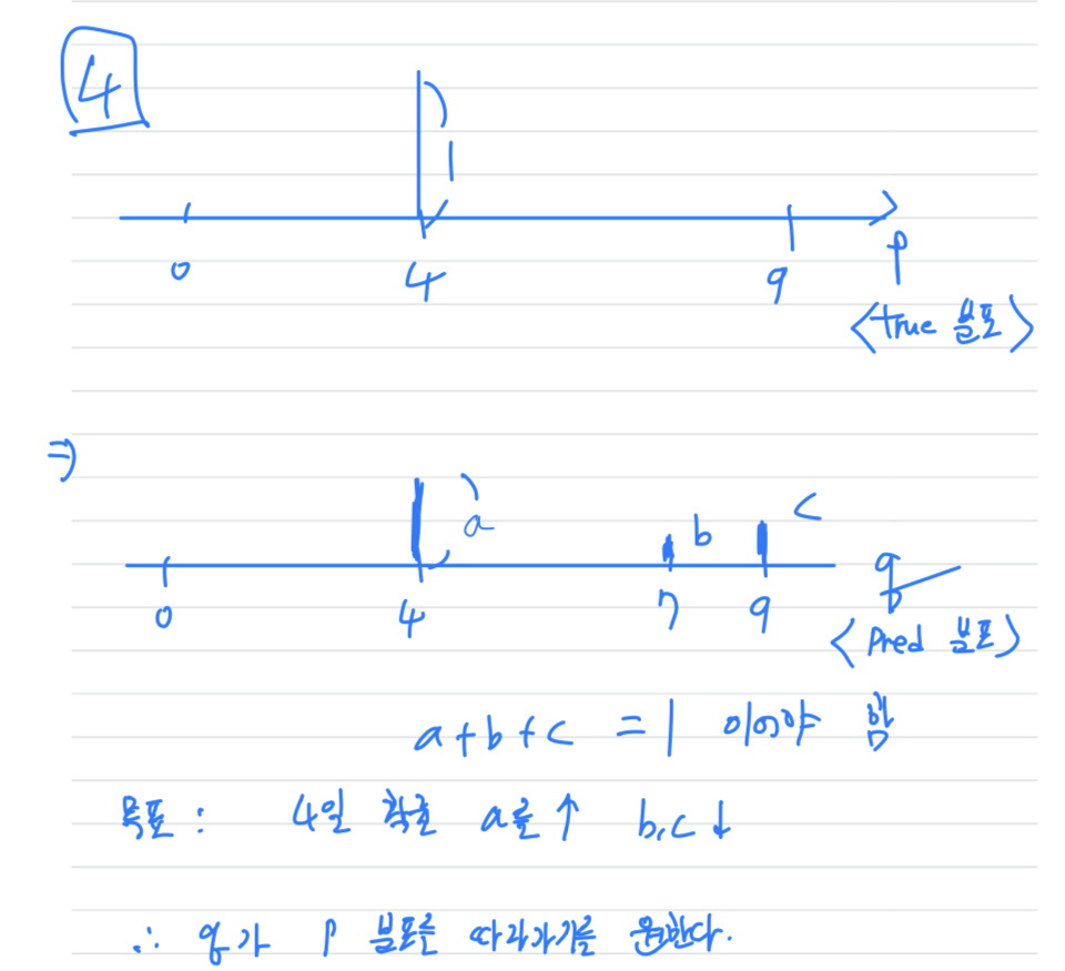
  Observed == True Distribution : $(p, 1-p)$
  Fitted == Predicted Distribution : $(q, 1-q)$
  서로 다른 두 분포에 대한 불확실성.
  Cross Entropy를 줄여야 $q$가 $p$ 분포에 가까워짐
  

Alternative deriavtion based on cross entropy

• Negative log-likelihood(NLL)
  
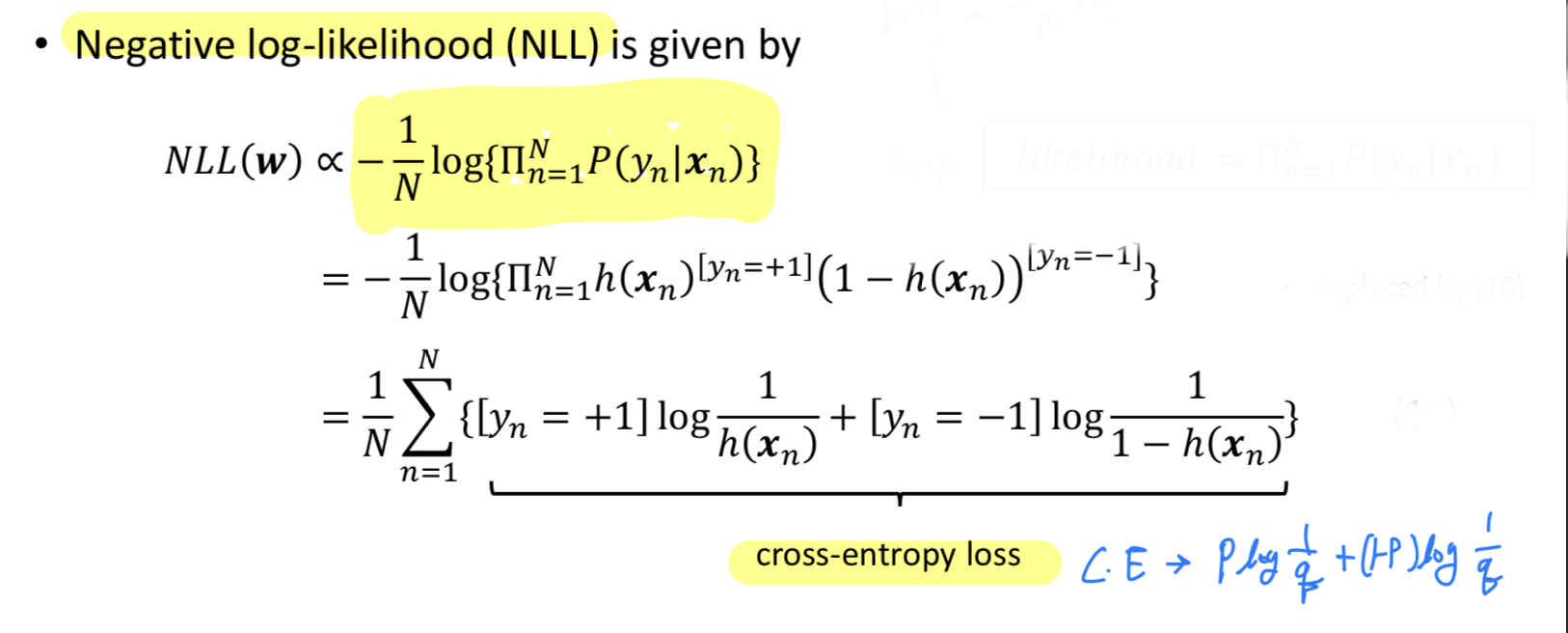
  • $p$ : target distribution
  • $q$ : prediction distribution

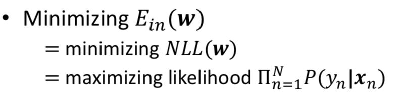
Training via Gradient Descent

• Logistic Regression : Minimize $E_{in}$ by setting $\Delta E_{in}(w)=0$
  ➡️ Iterative Optimization (e.g. Gradient Descent)

Gradient Descent

• General technique for minimizing twice-differentiable function (2번 미분 가능한 함수에 적용)
  

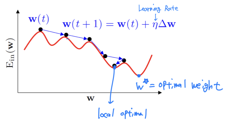
• Weight Update할 때, Two things to decide :

  1. Which Direction? ➡️ The Direction of Unit Vector : $||\hat v||$
  2. How Much? ➡️ Learning Rate : $\eta$
     
  • Learning Rate $\eta$는 Heuristic하게 정한다.
    하지만 일반적으로 Learning Rate가 너무 크거나, 너무 작으면 좋지 않다.
    적당해야 좋은 Learning이 이루어진다.
  • 그래서 초반에는 크게, 후반에는 작게 하여 효율적으로 학습을 진행하는 기법도 있다.

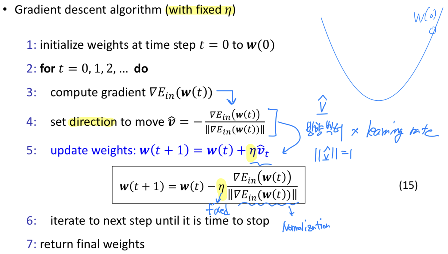
Logistic Regression Algorithm

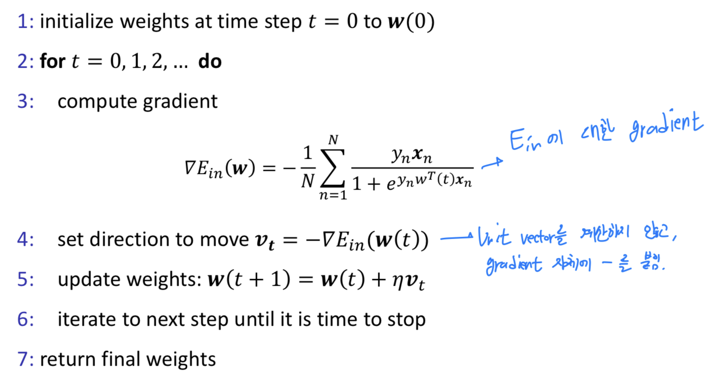
We have more loose ends to tie

1. How to choose initial weights $w(0)$
   ➡️ zeros로 초기화하는 것이 아니라, random하게 initialization하는 것이 좋다는 연구 결과
2. How to set the criterion for stopping gradient descent
   1) Large upper bound for the numbr of iterations
   2) Small lower bound for the size of gradient

Variants of gradient descent

• Batch gradient descent
  : Use all $N$ examples in each interation

• Stochastic gradient descent
  : Use 1 example in each iteration

• Mini-batch gradient descent
  : Use $b$ examples in each iteration ($b$ : mini-batch size (typically 2~100))