Paper Info

• author : Mark Sandler, Andrew Howard, Menglong Zhu, Andrey Zhmoginov, Liang-Chieh Chen
• Subjects : The IEEE Conference on Computer Vision and Pattern Recognition (CVPR), 2018, pp. 4510-4520

---

Abstract

• 이 논문에서 우리는 mobile model에 대한 다양한 task 뿐만 아니라 다른 model size spectrum에서도 state of the art performance를 보이는 new mobile architecture, MobileNetV2를 소개할 것이다.

• 우리는 또한 SSDLite라고 불리는 새로운 framework을 사용하여
  mobile model에 object detection을 적용하는 효율적인 방법을 소개할 것이다.

  • SSDLite :
    https://pytorch.org/vision/main/models/ssdlite.html
    https://pytorch.org/blog/torchvision-ssdlite-implementation/

• 추가적으로, 우리는 우리는 MobileDeepLabv3라고 부르는
  축소된 형태의 DeepLabv3를 통해 mobile semantic segmentation model을 만드는 방법을 설명할 것이다.

  • semantic segmentation이란 :
    사진에 있는 모든 pixel을 (미리 지정된 개수의)class로 분류하는 것
    (https://towardsai.net/p/l/machine-learning-7)

• MobileDeepLabv3은 inverted residual structure에 기초를 두고 있다.
  inverted residual structure는 얇은 bottlenectk layer 사이의 shortcut connection을 말한다.
  (기존의 residual block은 wide -> narrow -> wide structure with the number of channel.)
  (inverted residual block은 narrow -> wide -> narrow structure)

• The intermediate expansion layer uses
  lightweight depthwise convolutions to filter features as a source of non-linearity.
  Additionally,
  we find that it is important to remove non-linearities in the narrow layers
  in order to maintain representational power.

---

1.Introduction

• Neural network는 많은 분야에서 발전이 이루어지고 있다.
  하지만 현재의 state of the art network들은
many mobiles and embedded applications에 적용하기에
high computational resource가 필요하다.
  
  이 논문에서는 mobile이나 resource constrained environments를 위해 잘 맞춰진 neural network architecture를 소개할 것이다.
  우리의 Network는 same accuracy를 유지하면서
  the number of operations and memory needed를 줄이며 state of the art로 나아간다.

• Our main contribution is a novel layer module :
  the inverted residual with linear bottleneck.
  This module takes as an input a low-dimensional compressed representation which is first expanded to high-dimension and filtered with a lightweight depthwise convolution.
  그 다음에 feature들은 linear convolution을 통해 원래의 low-dimensional representation으로 돌아간다.
  
  정리 :
  The inverted residual with linear bottleneck block은 low-dimensional coompressed representation으로 압축된 input을
  high-dimension으로 확장시키고나서
  lightweight depthwise convolution을 통해 filter연산을 수행하여
  원래의 low-dimensional representation으로 되돌아간다.
  
  The official implementation is available as part of TensorFlow-Slim model library in https://github.com/tensorflow/models/tree/master/research/slim/nets/mobilenet
  

• 이 convolutional module은 특히 mobile design에 대해 적절하다.
  왜냐하면 이 module은 large intermidate tensor를 완전히 구현하지 않음으로써
  inference 동안 the memory footprint(=memory 사용량)이 크게 줄어든다.
  이를 통해 적은 양의 빠른 SW 제어 cache memory를 제공하는 많은 embedded HW 설계에서
  main memory access 필요성이 줄어든다.

---

2. Related Work

• accuracy와 performance 사이에 최적의 balance를 위한 deep neural architecture에 대한 연구가
  지난 몇 년간 활발히 이루어지고 있다.
  
  manual architecture search와 improvement in training algorithm (AlexNet, VGGNet, GoogLeNet, ResNet) 뿐만 아니라
  hyper parameter optimization method(Random search for hyper-parameter optimization, bayesian optimization, 등),
  network pruning(12 ~ 17) and connectivity learning(18, 19) 에도 많은 발전이 있었다.
  
  ShuffleNet 또는 introducing sparsity와 같이
  internal convolution block의 connectivity structure를 변화시키는 것이 최근 활발히 연구되어지고 있다.
  
  최근에 genetic algorithm과 reinforcement learning에 대한 architectural search를 포함하여
  optimization method에 대한 새로운 방향들이 소개되어지고 있다.
  하지만 한가지 단점으로, 결과적인 network가 매우 복잡해진다는 것이다.

• 이 논문에서,
  우리는 neural network가 어떻게 작동하는지에 대한 better intuition을 개발하고
  가능한 simplest network design 설계를 돕는 데에 사용하는 것을 목표로 한다.

• Our network design is based on MobilNetV1.
  우리의 network는 simplicity를 유지하고, accuracy를 향상시키는 동안에 어떠한 special operator들이 필요하지 않다.

---

3. Preliminaries, discussion and intuition

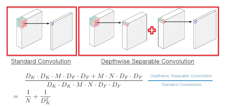
3.1 Depthwise Separable Convolutions

• Depthwise Separable Convolutions은 많은 efficient neural network architecture(27, 28, 20)들의 핵심적인 building block이고,
  우리는 또한 이번 연구에 depthwise separable convolutions을 사용했다.
  The basic idea는 a full convolutional operator를
  2개의 separate layer로 나눈 factorized version으로 교체하는 것이다.
  

1. 첫번째 layer는 depthwise convolution이라고 불리고,
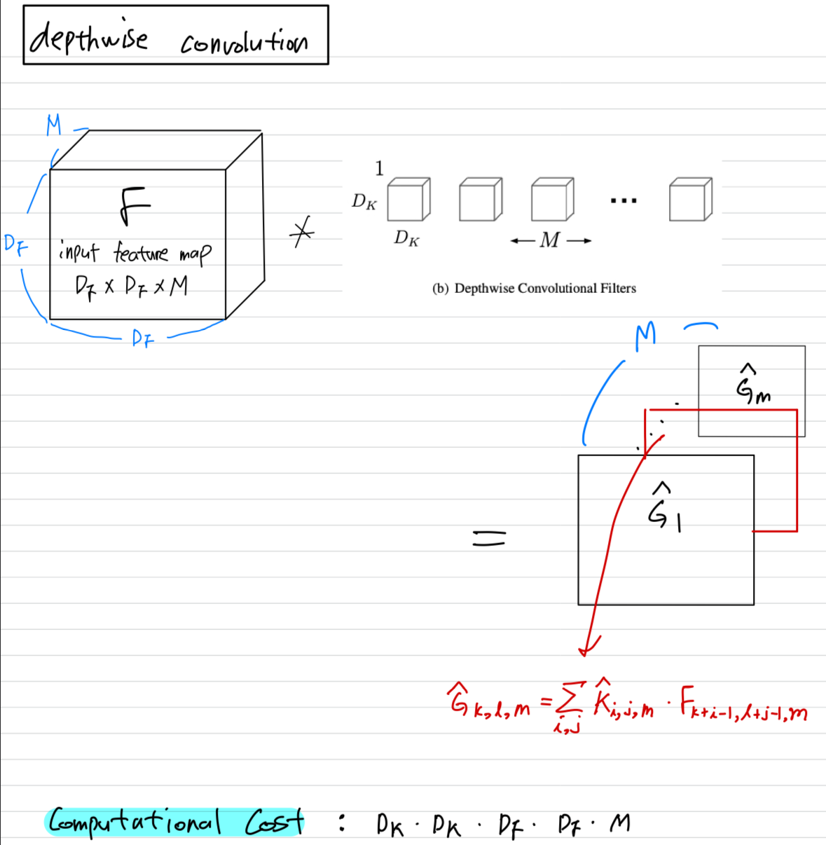
   input channel 마다 single convolutional filter를 적용함으로써 lightweight filtering을 수행한다.
2. 두번째 layer는 pointwise convolution이라고 불리고,
   1x1 convolution을 한다.
   그리고 input channel의 linear combination computing을 통해 새로운 feature를 만들어낸다.

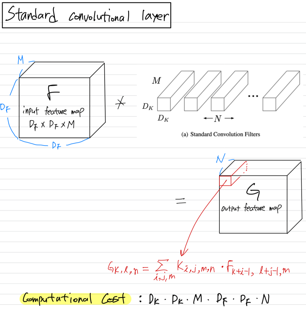
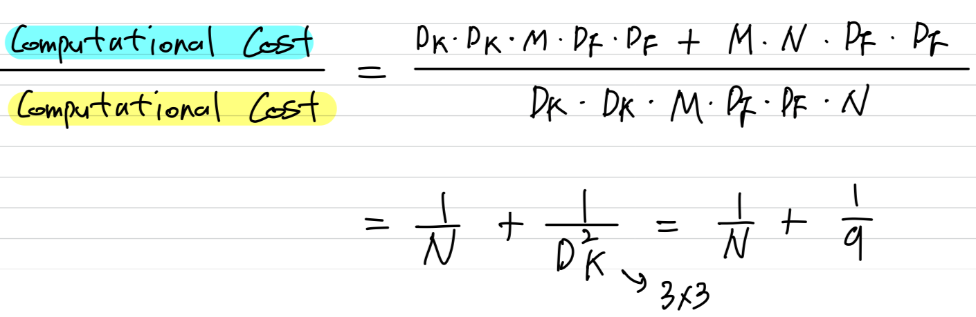
• Standard convolution takes an $h_i$ x $w_i$ x $d_i$ input tensor $L_i$,
  and applies convolutional kernel $K \in R^{k * k * d_i * d_j}$ to produce an $h_i$ x $w_i$ x $d_j$ output tensor $L_j$.
  The computational cost of $h_i * w_i * d_i * d_j * k * k$.

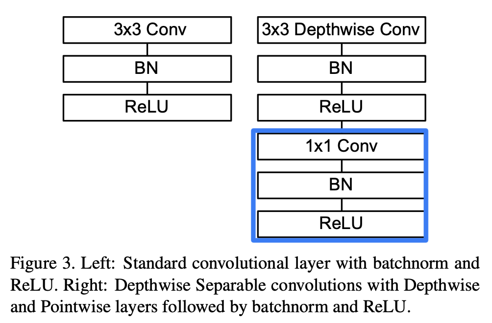
MobileNetV1에서 설명한 Depthwise Separable Convolution

• Depthwise Separable Convolution :
  MobileNet model은 depthwise separable convolution으로 이루어져 있다.
  depthwise separable convolution은
  depthwise convolution과 pointwise convolution이라고 불리는 1x1 convolution으로 이루어져 있다.
  1. depthwise convolution applies a single filter to each input channel.
  2. pointwise convolution applies a 1x1 convolution to combine the outputs the depthwise convolution.
• Standard convolutional layer takes as input a $D_F$ X $D_F$ X $M$ feature map $F$ and
  produces a $D_F$ X $D_F$ X $N$ feature map $G$
  where $D_F$ is the spatial width and height of a squre input feature map,
  $M$ is the number of input channels,
  $D_G$ is the spatial width and height of a square output feature map and $N$ is the number of output channel.
  

• Depthwise Separable convolution
  1. depthwise convolution :
     We use depthwise convolutions to apply a single filter per each input channel (input depth).
     
  2. pointwise convolution :
     1×1 convolution, is then used to create a linear com- bination of the output of the depthwise layer.
     

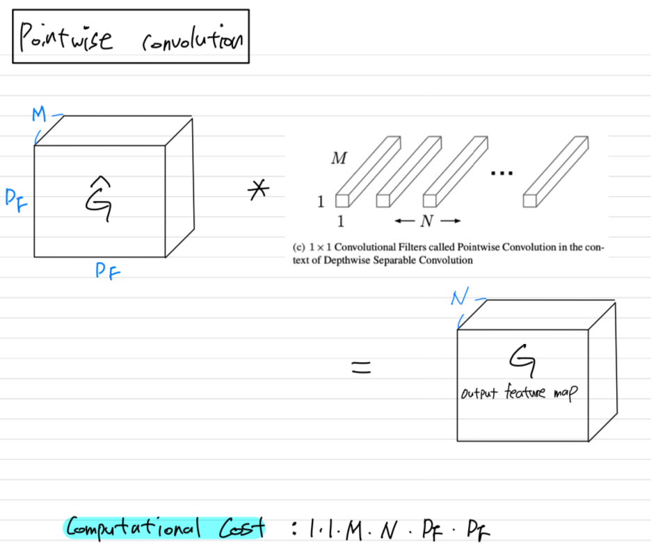
• By expressing convolution as a two step process of filtering and combining we get a reduction in computation of :
  

Summary (https://www.youtube.com/watch?v=JuEeRdRG_2E)

3.2 Linear Bottlenecks

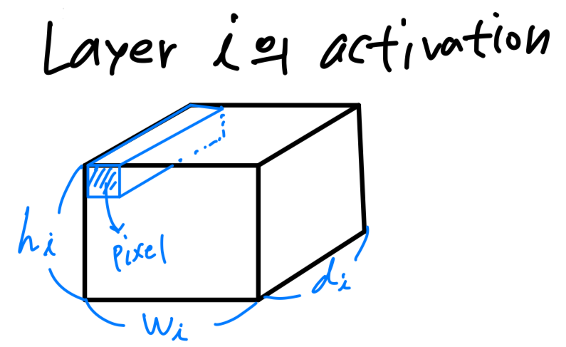
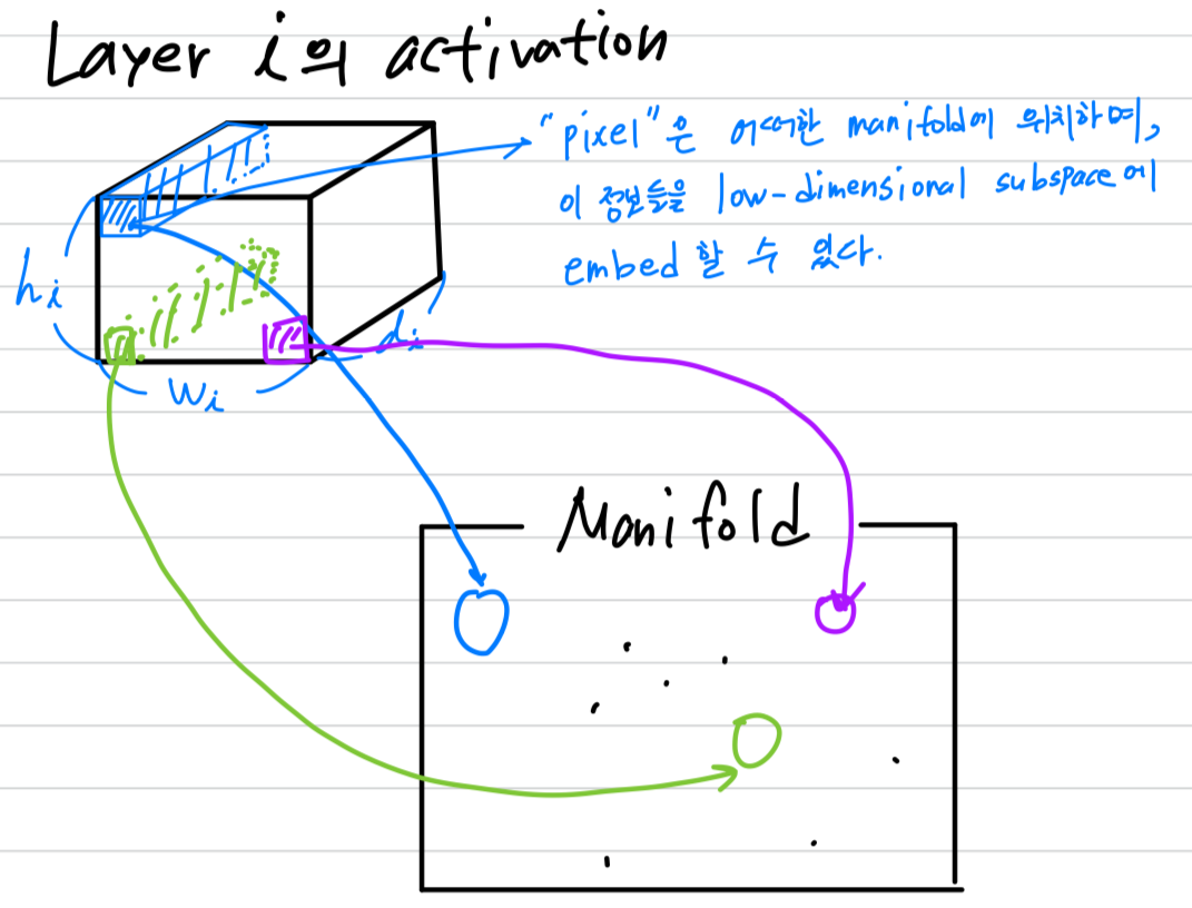
• $n$개의 layer $L_i$로 구성되어 있는 deep neural network를 고려하자.
  각 layer의 activation은 $h_i$ x $w_i$ x $d_i$ 를 갖는다.
  
  이 section에서는 $h_i$ x $w_i$ x $d_i$ 라는 tensor의 property에 대해서 살펴볼 것이고,
  이는 $d_i$차원을 갖는 pixel이 $h_i$ x $w_i$개 있다고 생각할 수 있다.
  

• real image에 대한 input set에 대해서,
  우리는 이러한 set of layer activations이 "manifold of interest" (관심영역에 대한 manifold)를 형성한다고 말할 수 있다.
  neural network에서 mainfolds of interest가 low-dimensional subspace로 embedded될 수 있다고 가정되어 왔다.
  
  즉, 모든 독립적인 d-channel pixel을 볼 때,
  encode되어 있는 정보는 어떠한 manifold 상에 위치하며, 그 정보들을 저차원의 subspace로 보낼 수 있다는 것이다.
  

• 언뜻 보기에, 이러한 사실은 단순히 layer의 차원을 줄임으로써 운영될 수 있다.
  MobileNetV1에서는 width multiplier parameter로 computation과 accuracy의 tradeoff를 효율적으로 다루며 성공적으로 사용되었다.
  
  이 직관을 따르면,
  width multiplier 접근법은 manifold of interest가
  전체 공간에 걸쳐 있을 때까지 activation space의 차원을 줄일 수 있을 것이라 생각된다.
  
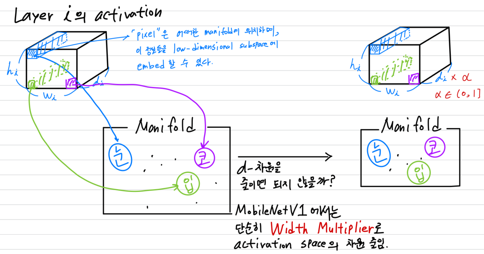
  하지만 이러한 직관은 deep convolutional neural network가 실제로
  ReLU와 같은 nonlinear coordinate transformation(좌표 변환)을 갖고 있기 때문에 깨지게 된다.
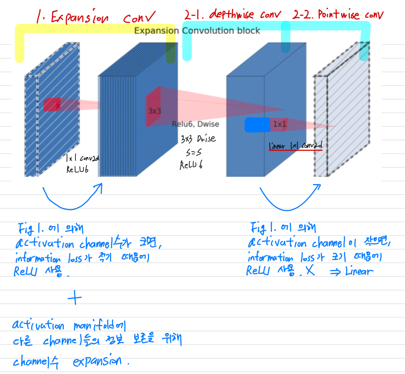
  (Figure 3.은 MobileNetV1에서 pointwise convolution에서 ReLU nonlinearity를 사용한 모습이다.)
  
  ReLU가 channel을 붕괴시키면, 해당 channel에 대한 정보가 손실될 수 밖에 없다.
  ➡️ (1) 따라서 V2의 pointwise convolution에서는 ReLU를 사용하지 않고 Linear 연산만 수행함.
  ReLU Nonlinearity를 추가한 network와 추가하지 않고 Linear 연산만한 network의 performance 비교 :
  
  
  
  그리고 ReLU에 사용되는 activation channel이 많다면, activation manifold에는 다른 channel의 정보가 계속해서 보존될 수 있는 구조가 된다.
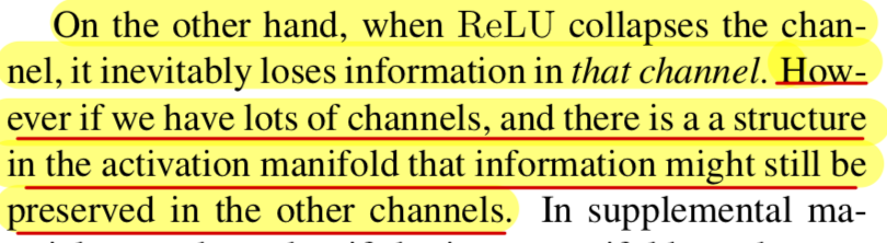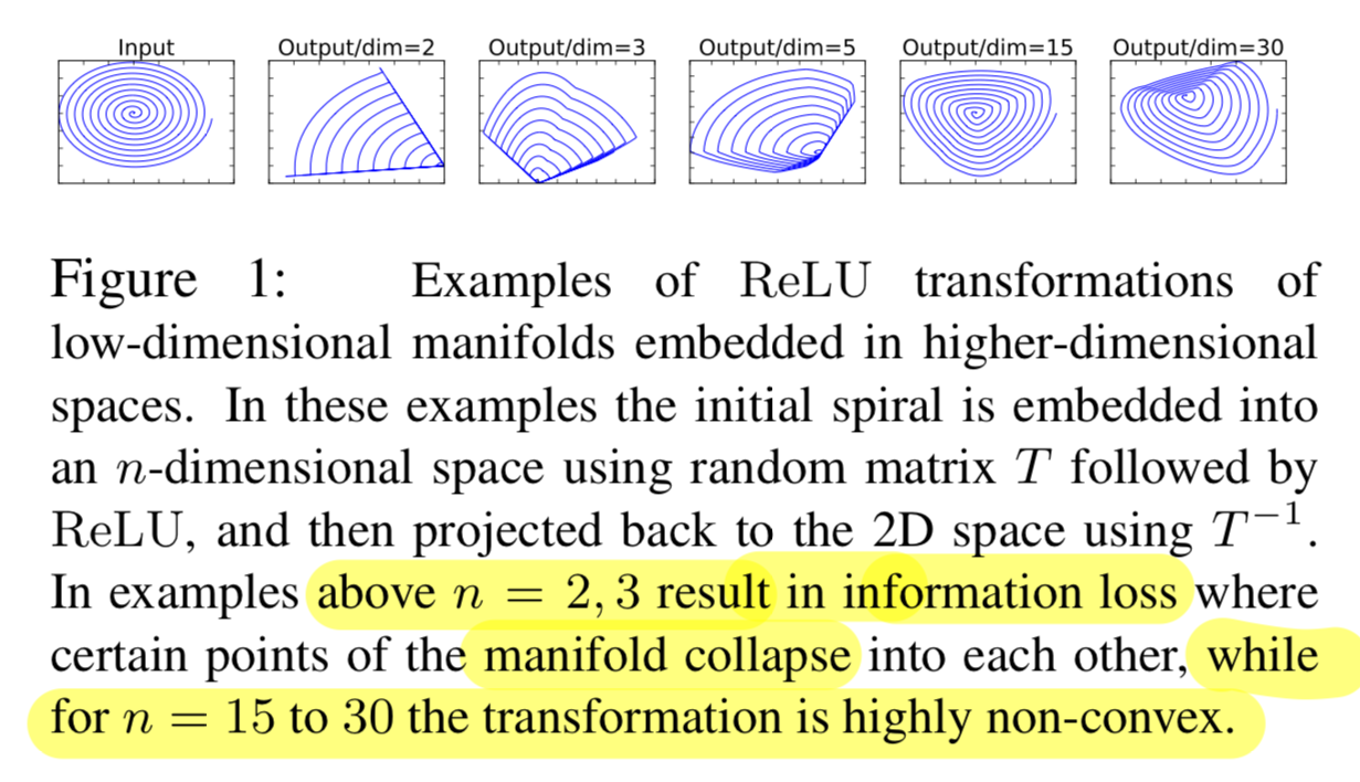
  Figure 1에서 출력 channel이 작은 경우에 정보가 손실되고, 크면 클수록 정보를 보존한다는 것을 실험적으로 보임.➡️ (2) 따라서 V2의 depthwise convolution을 하기 전에 expansion layer를 추가
  
  

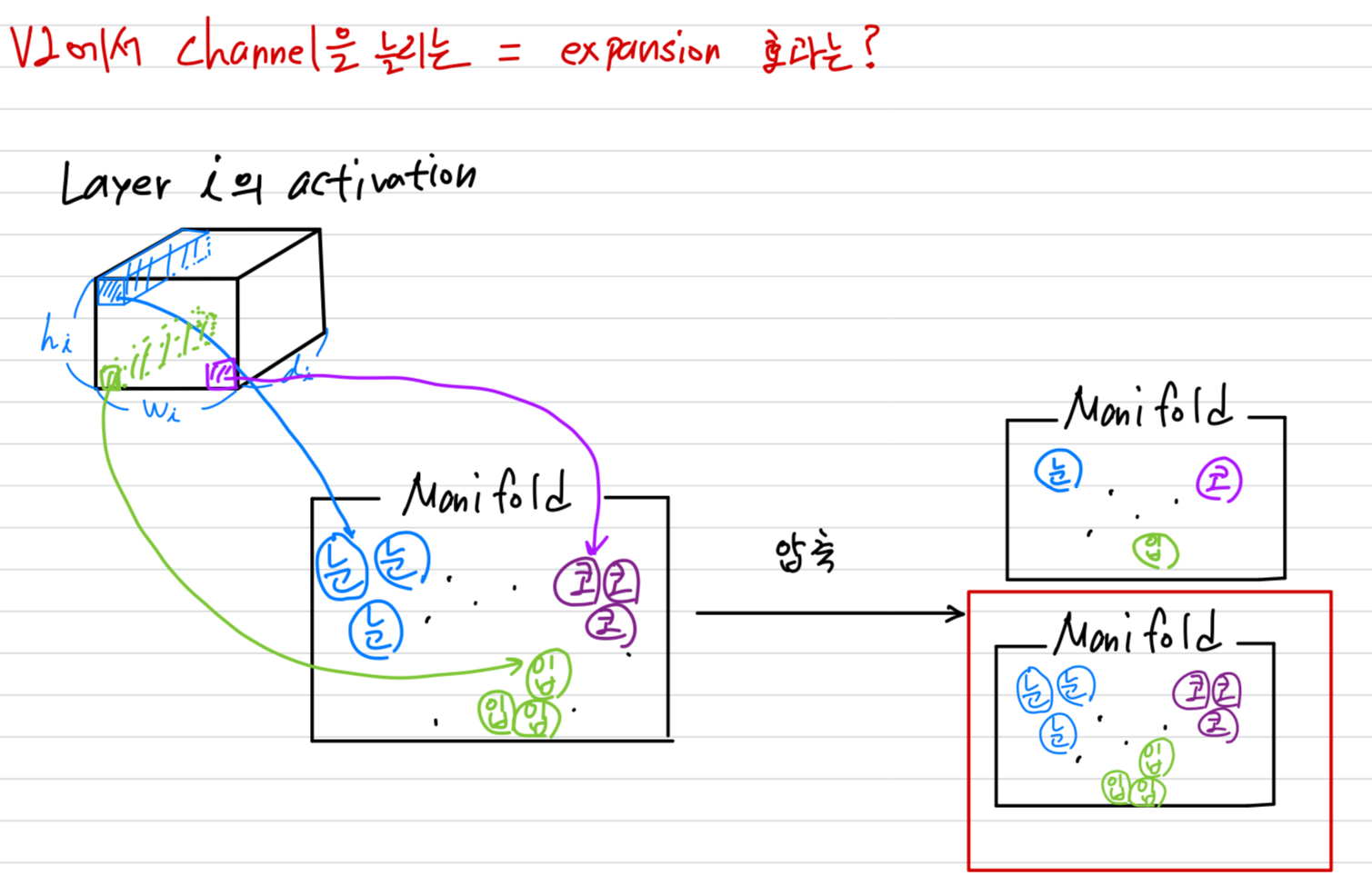
  (내 생각, 비유)
  큰 도화지(manifold)에 작은(depth) 고양이를 그려서 구기고, 이를 펼치는 것보다
  작은 도화지(manifold)에 큰(depth) 고양이를 그려서 구기고, 이를 펼치는 것이
  고양이를 분류하는 데에 더욱 쉬울 것이다. (학습이 더 잘 될 것이다.)
  

• 요약하자면,
  우리는 manifold of interest가 higher-dimension activation space의 low-dimensional subspace에 있어야 한다는 요구사항을 나타내는 2가지 속성을 강조했다.
  1. If the manifold of interest remains non-zero volume after ReLU transformation,
     it corresponds to a linear transformation.
  2. ReLU is capable of preserving complete information about the input manifold,
     but only if the input manifold lies in a low-dimensional subspace of the input space.
     
     
     이 2가지 속성은 우리에게 optimizing existing neural architecture에 대한 hint를 제공했다.
     manifold of interest가 low-dimension에 있다고 가정하면,
     linear bottleneck layer를 convolutional layer에 삽입하여 이를 포착할 수 있을 것이다.
     이 논문의 나머지 부분에서,
     우리는 bottleneck convolution을 사용할 것이다.
     우리는 input bottleneck size와 내부 size 사이의 크기를 맞추는 비율을 expansion ratio라고 할 것이다.
     

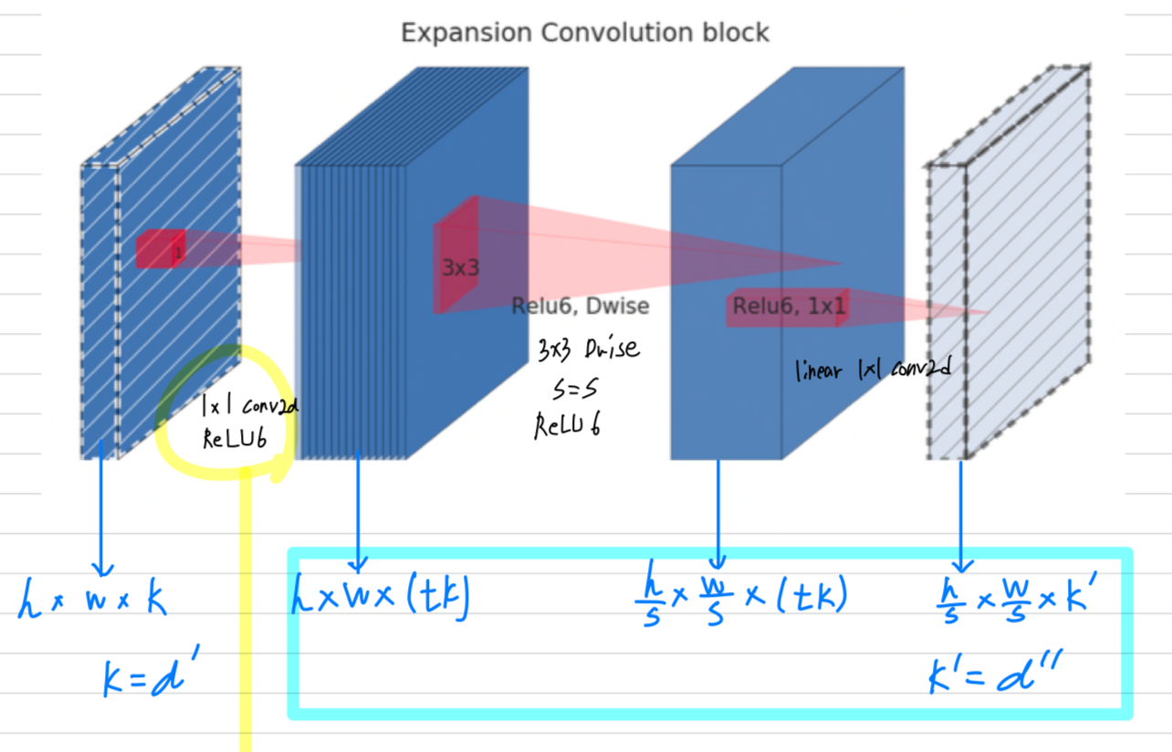
3.3 Inverted residuals

• bottleneck block은 residual block과 비슷한데,
  bottleneck은 expansion을 따르는 input을 갖는다.
  우리는 또한 gradient propagation ability를 향상시키기 위해
  bottleneck 사이에 shortcuts을 사용했다.
  
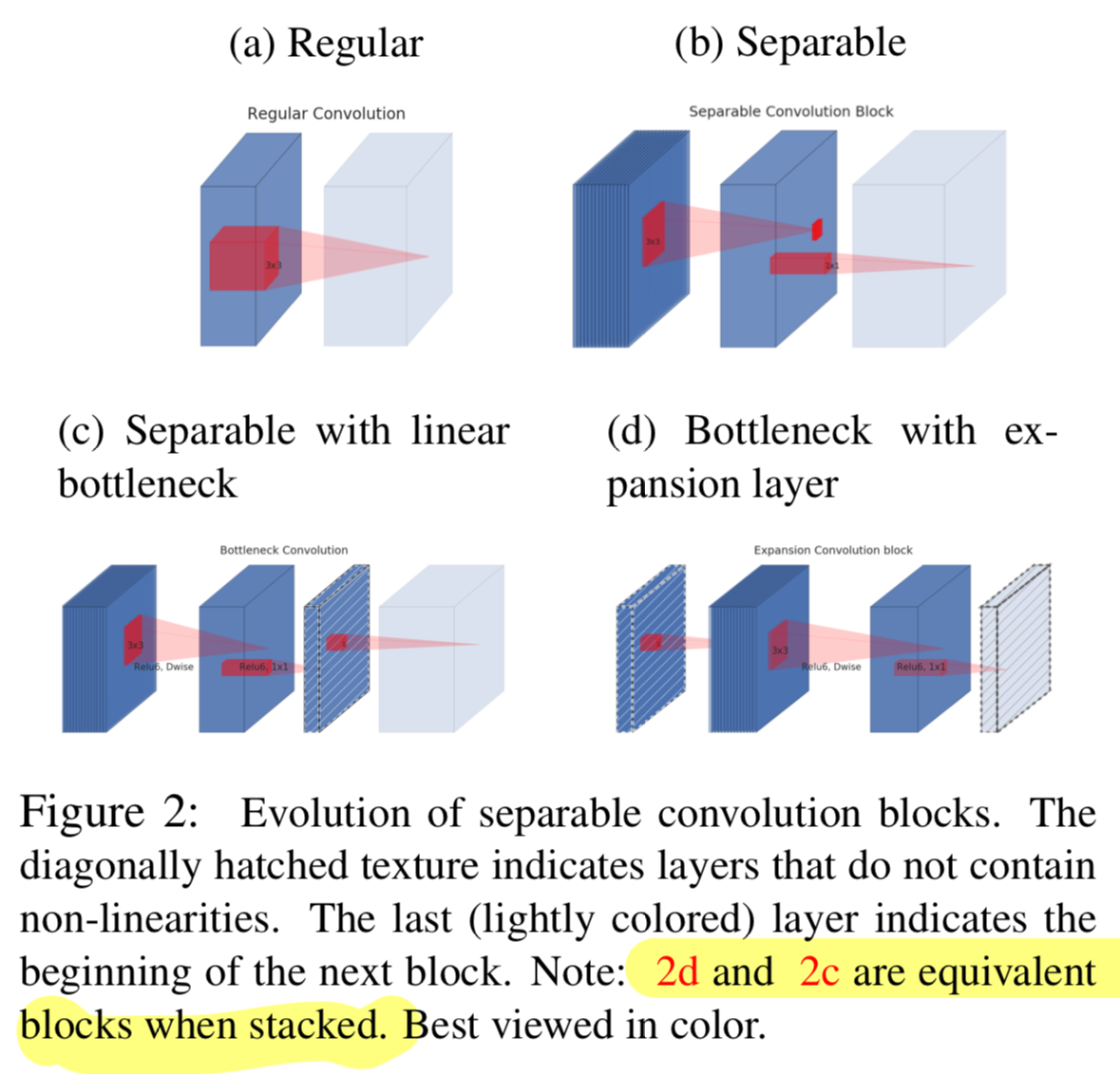
  기존의 (a) : Residual block은 wide-narrow-wide
  새로운 (b) : Inverted residual blcok은 narrow-wide-narrow
  

Running time and parameter count for bottleneck convolution

• Table 1 : The basic implementation structure.
  ReLU6 : $min(max(0,x),6)$
  For a block of size $h$ x $w$.
  expansion factor $t$ and kernel size $k$ with $d'$ input channel and $d''$ output channels,
  the total number of multiply add required is $h*w*d'*t(d'+k^2+d'')$
  

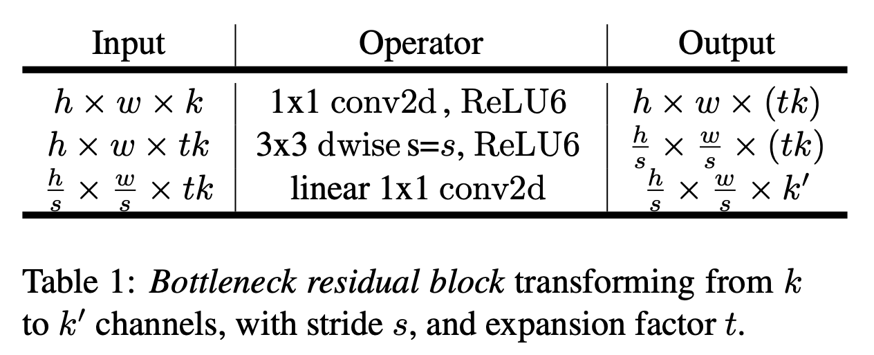
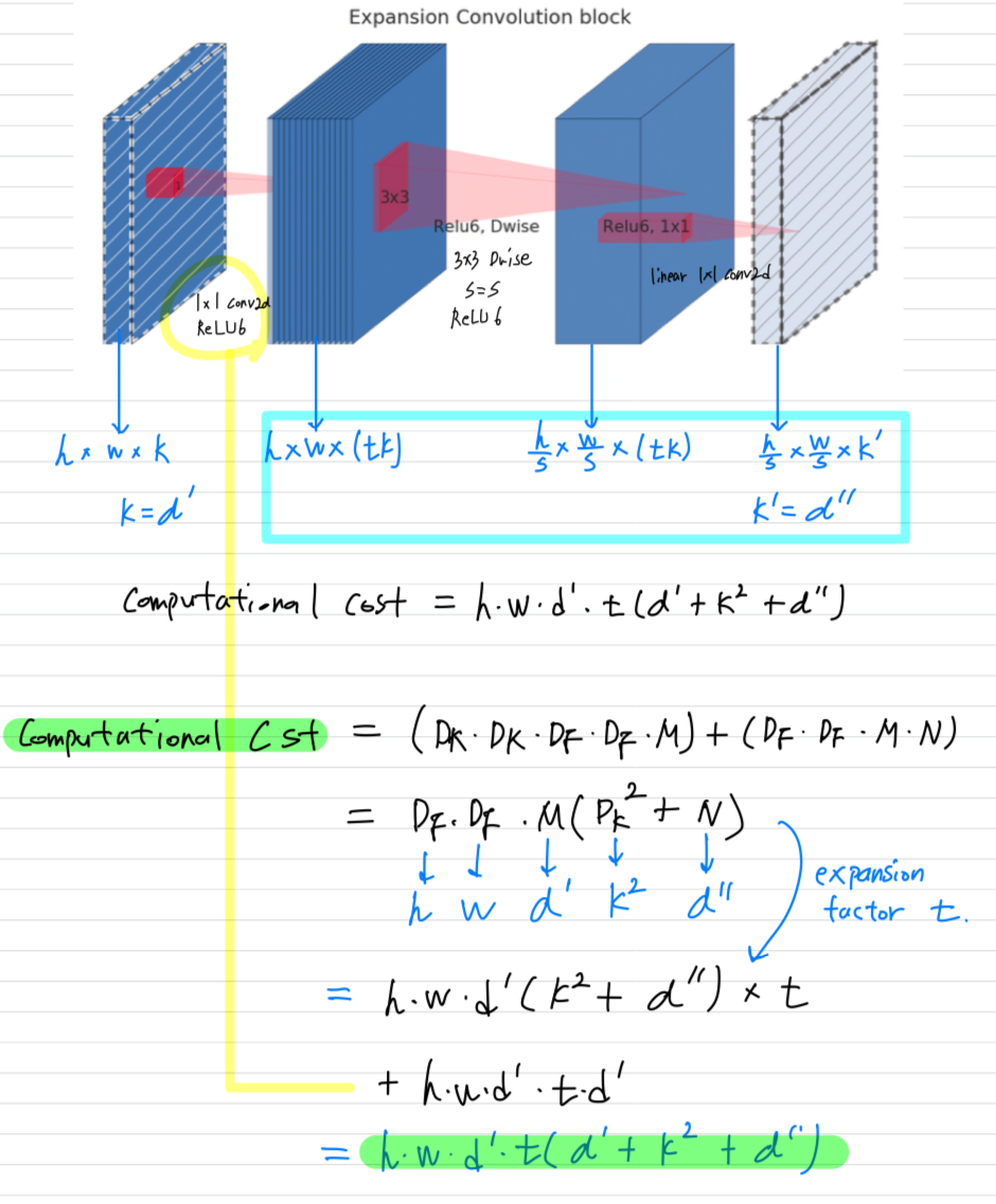
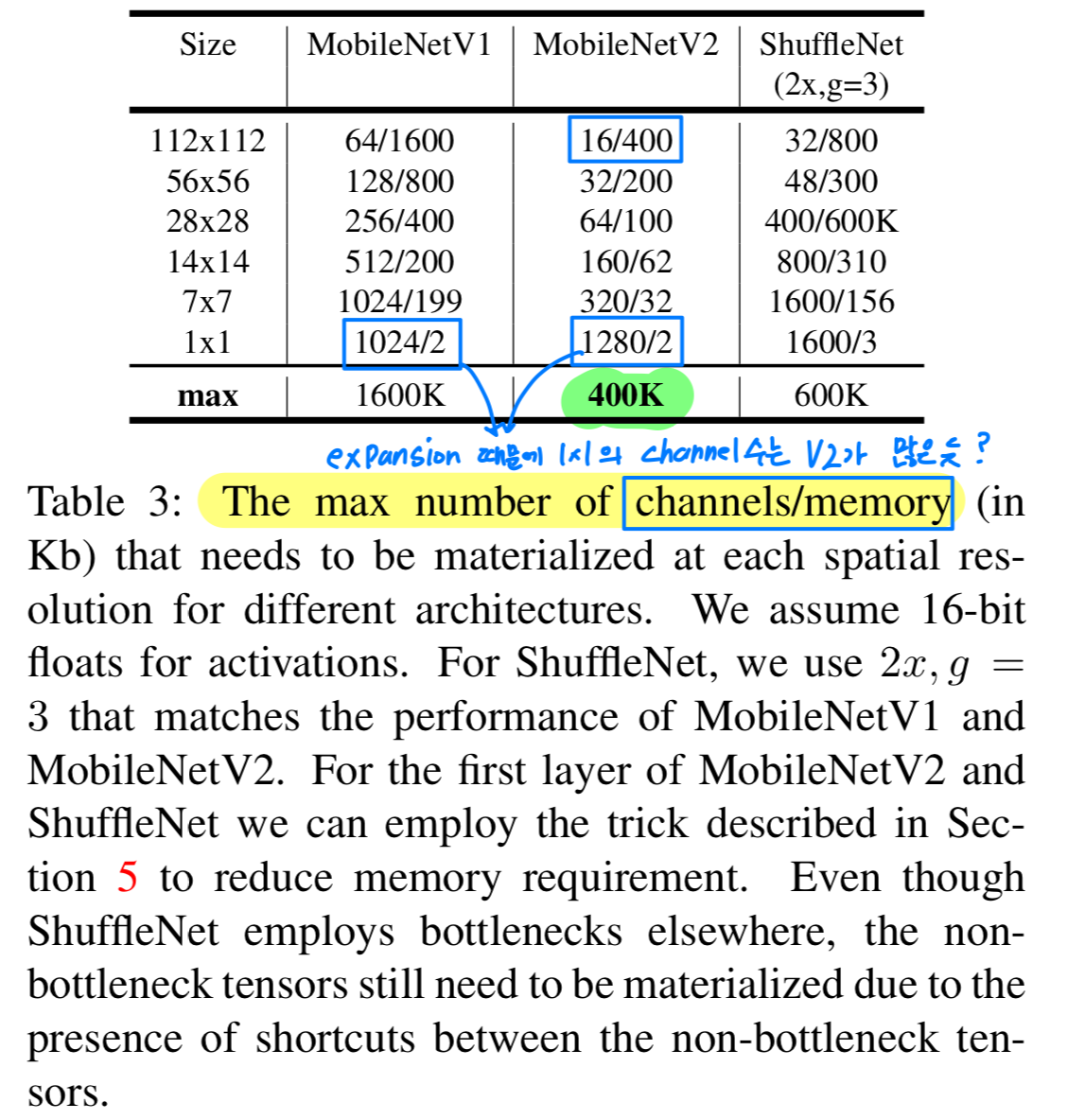
• Table 3 :
  We compare the needed sizes for each resolution
  between MobileNetV1, MobileNetV2, ShuffleNet.
  

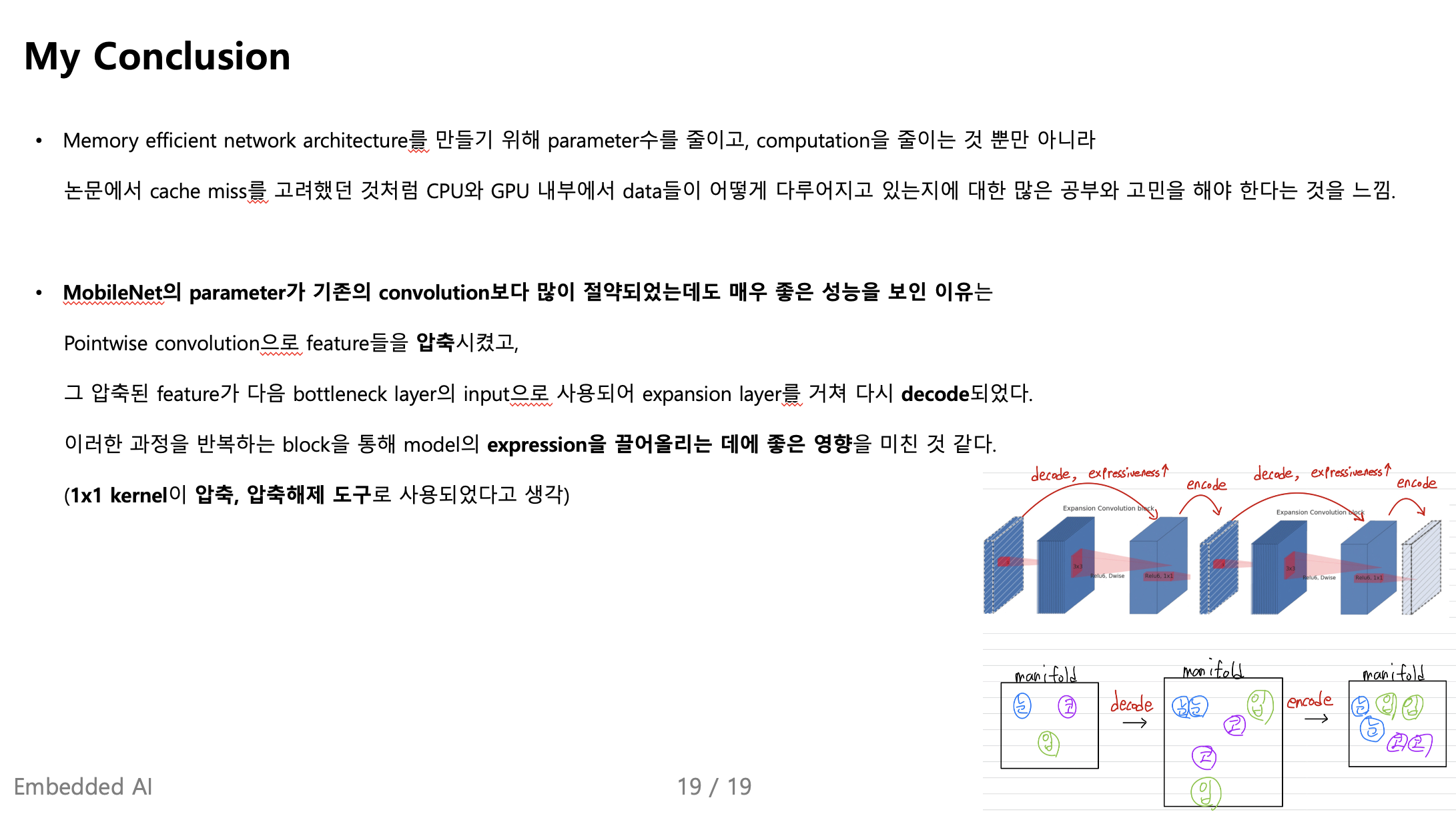
3.4 Information flow interpretation

• architecture의 한 가지 흥미로운 특성은
  bottleneck layer의 input/output domain과
  input을 output으로 변환하는 nonlinear function 사이의
  자연스러운 separation(분리)를 제공한다는 것이다.
  전자(bottleneck layer의 input/output domain)은 각 layer의 capacity로 볼 수 있고,
  후자(input을 output으로 변환하는 nonlinear function)은 expressiveness로 볼 수 있다.
  
  이는 이전의 capacity와 expressiveness가 얽혀있던 traditional convolution block과는 대조된다.
  
  우리의 경우,
  inner layer depth를 0으로 할 때, shortcut connection으로 인해 기본적인 convolution은 identity function이 된다.
  expansion ratio를 1보다 작게 할 때, 이는 classical residual convolutional block이 된다.
  하지만 우리의 목적을 위해 우리는 expansion ratio를 1보다 크게 하여 사용했다.
  
  이 해석을 통해
  network의 expressiveness와 capacity를 분리하여 연구할 수 있으며,
  network 속성에 대한 더 나은 이해를 제공하기 위해 이러한 분리에 대한 추가적인 탐구가 필요하다고 생각한다.

network의 expressiveness는 expansion layer에서 channel수를 얼만큼 늘려주느냐에 따라 결정되고,
capacity는 projection(pointwise layer)에서 channel수를 얼만큼 줄이느냐에 따라 결정된다.
따라서 실제로 expressiveness를 계산하는 것은 depthwise convolution에서 수행되고,
expansion, projection에서 capacity를 조절하는 역할을 하기 때문에
하나의 block에서 expressiveness와 capacity가 분리되어 있어서
따로따로 control할 수 있게 만들었다고 해석...

---

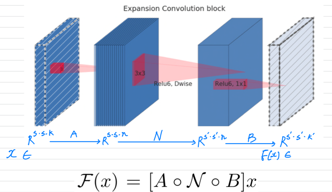
4. Model Architecture

• 이제 architecture에 대한 detail을 설명할 것이다.
  이전 section에서 설명한 the basic building block은
  residual이 있는 bottleneck depth-separable convolution이다.
  
  The detailed structure of this block is shown in Table 1.
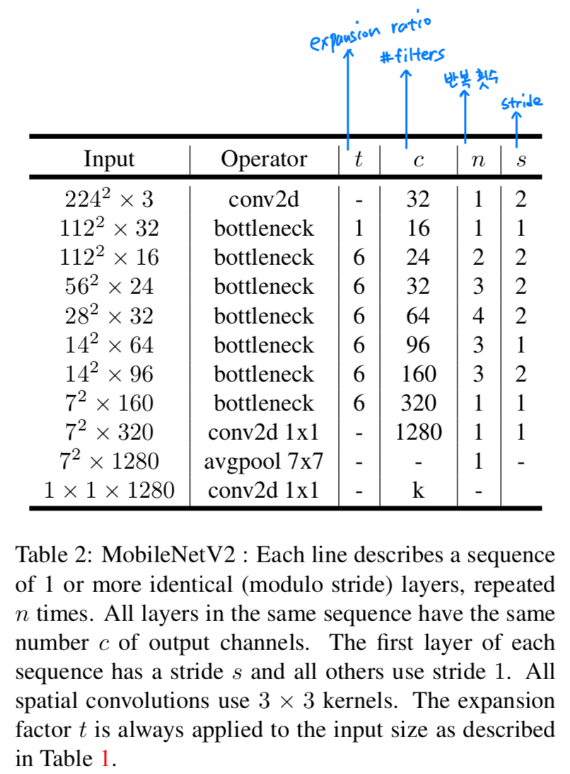  The architecture of MobileNet2 contains the initial fully convolution layer with 32 filters,
  followed by 19 residual bottleneck layers described in the Table 2.
  We use ReLU6 as the non-linearity because of its robustness when used with low-precision computation.
  We always use kernel size 3 x 3, and utilize dropout and batch normalization during training.
  first layer를 제외하고, 우리는 고정적인 expansion rate를 사용했다.
  실험상 우리는 expansion rate가 5~10인 것이 좋다고 발견했다.
  상대적으로 작은 network에는 더 작은 expansion rate, 상대적으로 큰 network에는 더 큰 expansion rate를 사용하는 것이 좋다고 발견했다.
  we use expansion factor of 6 applied to the size of the input tensor.
  예를 들어, 64-channel을 input tensor로 갖고 128-channel을 output tensor로 갖는 layer에서
  intermediate expansion layer는 $64*6=384$ channels을 갖는다.

---

5. Implementation Notes

5.1 Memory efficient inference (?)

• TensorFlow나 Caffe를 사용하는 일반적인 inference implementation은
  directed acyclic compute hypergraph G를 만드는 것이다.
  G는 operation을 나타내는 edge와 intermediate computation을 나타내는 node로 구성되어 있다.
  Computation은 memory에 저장되어야 할 tensor들의 총 개수를 최소화하기 위해 schedule되어 진다.
  
  $R(i, \pi, G)$은 $\pi_i...\pi_n$ nodes들이 연결되어 있는 intermediate tensor의 list이다.
  $|A|$는 tensor $A$의 size이다.
  $size(i)$는 operation $i$ 동안에 내부 storage를 위해 필요한 memory의 총량이다.
  일반적으로
  그럴듯한 computation 조합인 $\Sigma(G)$을 탐색하고, $M(G)$를 minimize하는 것을 찾는다.

• residual connection과 같이 사소한 parallel structure만 있는 graph의 경우,
  사소하지 않은 계산 순서(residual connection)가 하나뿐이므로
  computation graph $G$에 대한 inference 단계에서 필요한 memory의 총량과 boundary를 단순화할 수 있다 .
  다시 말하면,
  memory의 총량은 모든 operation의 input과 output을 결합한 maximum total size로 단순화할 수 있다.
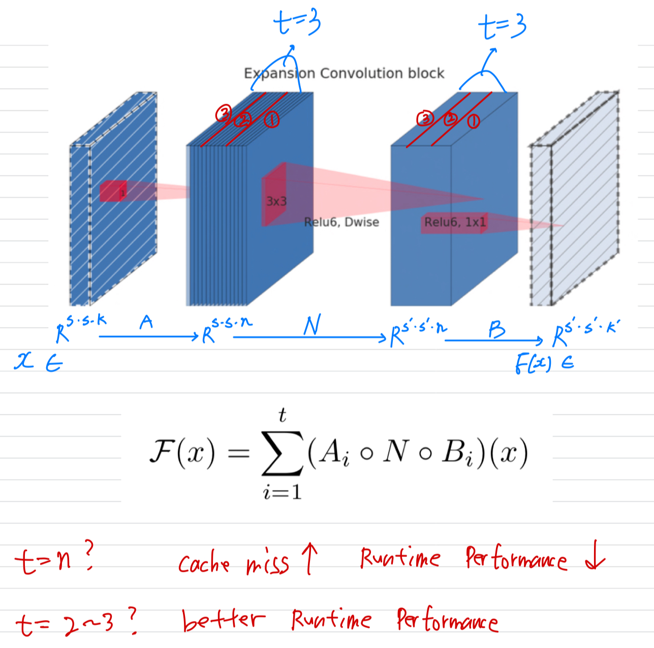
  우리가 bottleneck residual block을 하나의 single operation으로 취급하기 때문에
  memory의 총량은 bottleneck tensor의 size로 지정될 수 있다.
  

Bottleneck Residual Block

• Figure 3b에 있는 a bottleneck block operator $F(x)$는 다음의 3가지 operator의 구성으로 나타낼 수 있다.
  $A$는 Linear transformation이다. $A$ : $R^{s * s *k}$ -> $R^{s*s*n}$
  $N$은 nonlinear per-channel transformation이다. $N$ : $R^{s*s*n}$ -> $R^{s'*s'*n}$
  $B$는 output domain에 대한 linear transformation이다. $B$ : $R^{s'*s'*n}$ -> $R^{s'*s'*k'}$
  For our network $N=ReLU6 * dwise * ReLU6$ 이지만,
  output은 per-channel transformation을 적용한다.
  input domain size를 $|x|$, output domain size를 $|y|$라고 가정하면,
  $F(x)$를 계산하기 위해 필요한 memory는 최소한 $|s^2k| + |s'^2k'| + O(max(s^2, s'^2))$보다 작다.
  
  이 알고리즘은 inner tensor $I$가 $t$ tensor의 concatenation으로 표현될 수 있다는 사실에 기초를 두었고,
  각 $n/t$와 우리의 function은 다음과 같이 sum을 누적함으로써,
  size $n/t$의 intermediate block 하나만 memory에 항상 저장하기를 요구한다.
  이러한 trick을 사용할 수 있도록 하는 2가지 제약조건이 있다.

1. nonlinearity와 depthwise를 하는 inner transformation이 있다는 사실.
2. 연속적인 non-per-channel operator가 input size에서 output size에 대한 중요한 ratio를 갖는다는 것.
   
   $t$-way split을 사용하여 $F(x)$를 계산하는 데 필요한 multiply-adds operators의 수는 $t$와 무관하지만,
   기존 구현에서 하나의 matrix multiplication을 여러 개의 작은 multiplications로 대체하면
   cache miss가 증가하여 runtime performance가 저하된다는 것을 알 수 있다.
   우리는 $t$가 2~5 사이의 작은 상수일 때 가장 유용하다는 것을 알 수 있다.

정리 :
intermediate representation의 channel $n$이 있을 때,
$t=n$이라고 하면, 하나의 channel씩만 통과한다.
이는 cache miss로 인해 runtime performance가 안 좋다고 한다.
따라서 $t$를 작게 하여 intermediate representation을 보다 적은 tensor로 나누어 연산을 진행해야 한다.
실험상 $t$는 2~5가 좋다고 한다.

---

6. Experiments

6.1 ImageNet Classification

Training step

• We train our models using TensorFlow.
• standard RMSPropOptimizer with both decay and momentum set to 0.9
• we use BN after every layer.
• standard weight decay is set to 0.00004
• MobileNetV1에서처럼 initial learning rate of 0.045, decay rate of 0.98 per epoch.
• We use 16 GPU asynchronous workers, and a batch size of 96.

Results

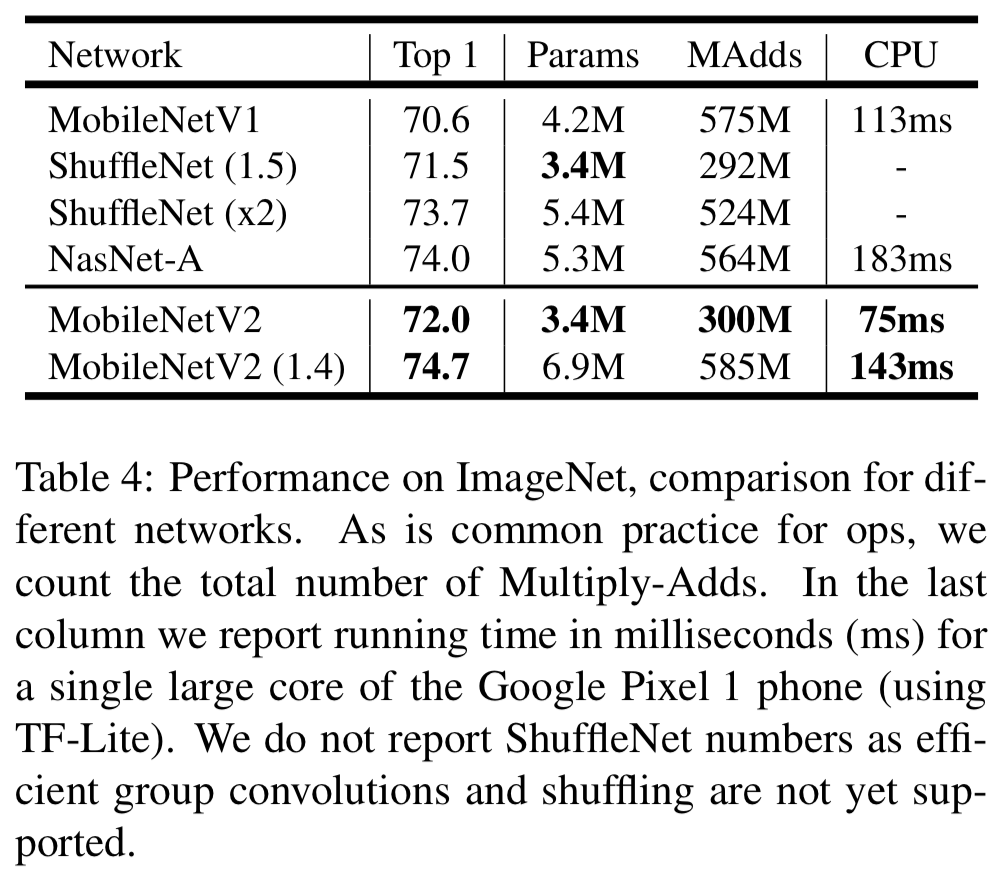
• MobileNetV2를 MobileNetV1, ShuffleNet, NASNet-A model과 비교했다.
  

6.2 Object Detection

• 우리는 COCO dataset에 대한 Single Shot Detector(SSD)의 수정된 version으로
  object detection에 대한 feature extractor로써 MobileNetV2와 MobileNetV1의 performance를 비교했다.
  우리는 또한 YOLOv2와 original SSD를 비교했다.

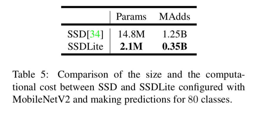
• SSDLite :
  이 논문에서,
  우리는 mobile에 사용할 수 있는 SSD의 또 다른 버전을 소개한다.
  우리는 모든 regular convolution을 separable convolutions(depthwise followed by 1x1 projection)으로 대체했다.
  이 design은 훨씬 더 computationally efficient하다.
  우리는 이 수정된 version을 SSDLite라고 한다.
  regular SSD와 비교했을 때, SSDLite는 급격하게 parameter 수와 computational cost를 줄였다. (Table 5)
  두 MobileNet model은 Open Source TensorFlow Object Detection API로 train되어졌다.
  두 model의 input resolution은 320 x 320로 했다.
  우리는 mAP(COCO challenge metrics), parameter 수, Multiply-Adds 수를 모두 benchmark하고 비교했다. (Table 6)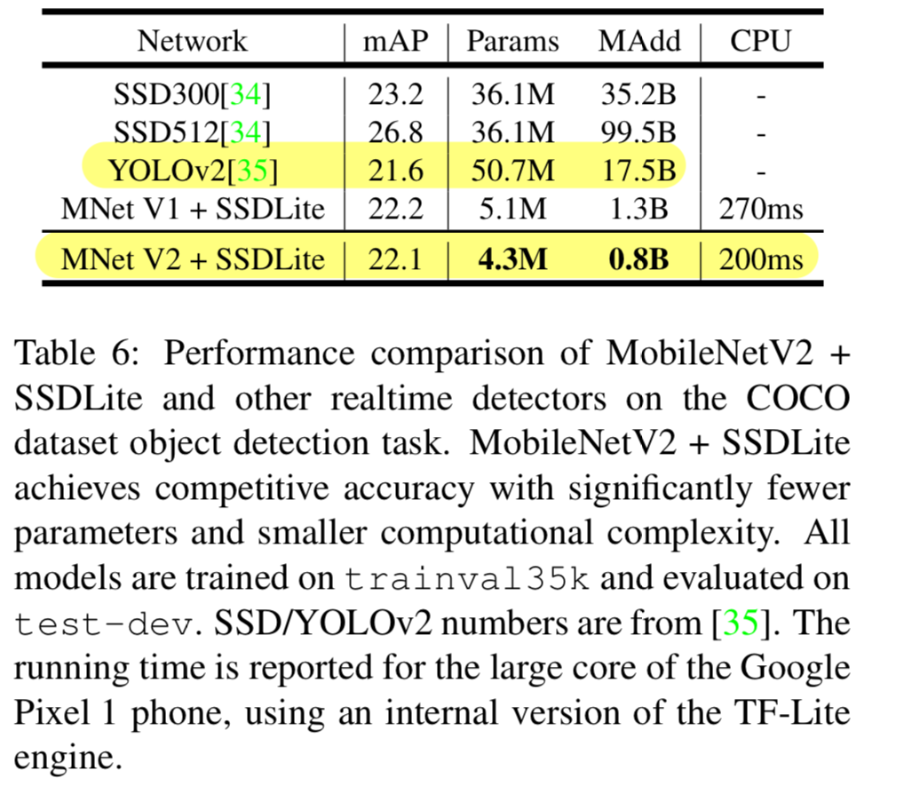주목할 만한 것은,
  MobileNetV2 SSDLite가 YOLOv2보다 20배 더 efficient하고 10배 더 작다.

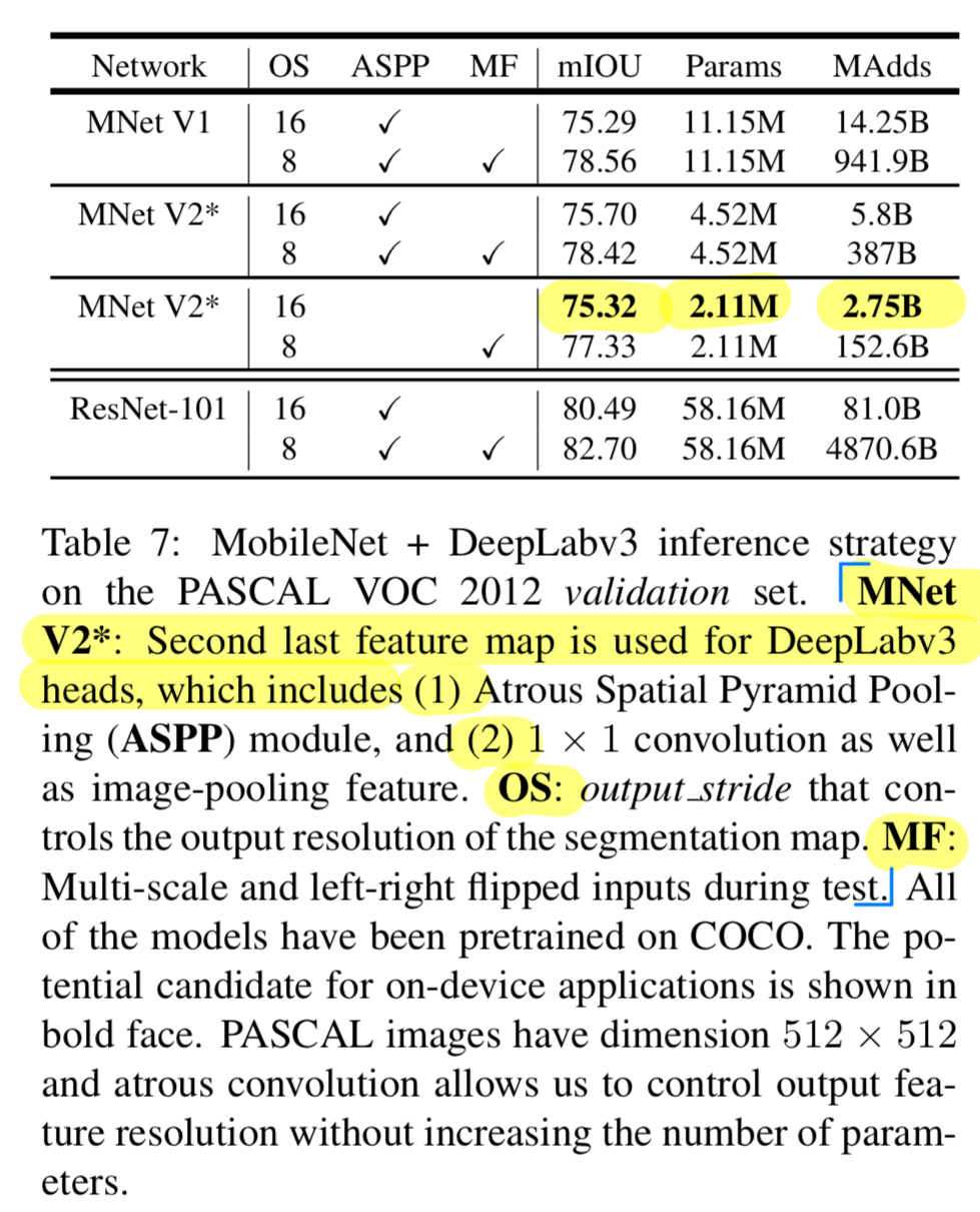
6.3 Semantic Segmentation

• 우리는 mobile semantic segmentation task를
  MobileNetV1과 MobileNetV2 model을 feature extractor로 사용하여
  DeepLabv3과 비교했다.

• DeepLabv3은 atrous convolution을 적용했고,
  계산된 feature map의 resolution을 control할 수 있는 강력한 tool이다.
  DeepLabv3에서 사용된 개념인
  (1) ASPP(Atrous Spatial Pyramid Pooling module)
  (2) OS : output stride that controls the output resolution of the segmentation map.
  과
  (3) MF : Multi-scale and left-right Flipped inputs during test.
  를 hyper parameter로 두고,
  evaluation metric mIOU에 대한 inference 진행.
  

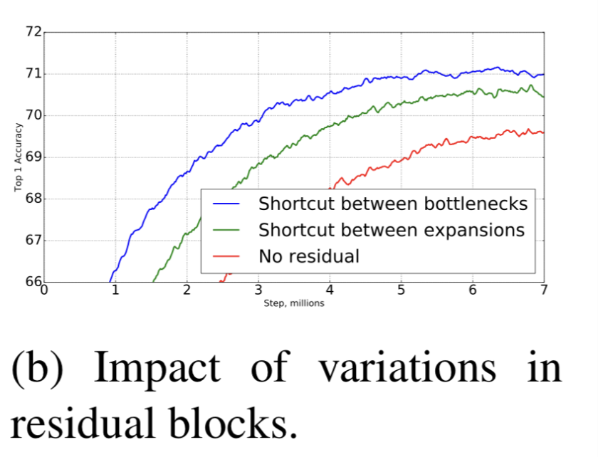
6.4 Ablation study

• Ablation study : 의학이나 심리학 연구에서, Ablation Study는 장기, 조직, 혹은 살아있는 유기체의 어떤 부분을 수술적인 제거 후에 이것이 없을때 해당 유기체의 행동을 관찰하는 것을 통해서 장기, 조직, 혹은 살아있는 유기체의 어떤 부분의 역할이나 기능을 실험해보는 방법

Inverted residual connections

• residual connection에 대한 중요도는 계속해서 연구되어지고 있다 [8, 30, 46]
  이 논문에서 bottleneck에 연결한 shortcut이
  expanded layer에 연결한 shortcut 보다 성능이 좋다는 것을 보여주고 있다. (Fig 6b)
  

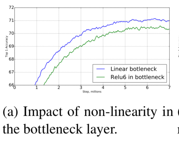
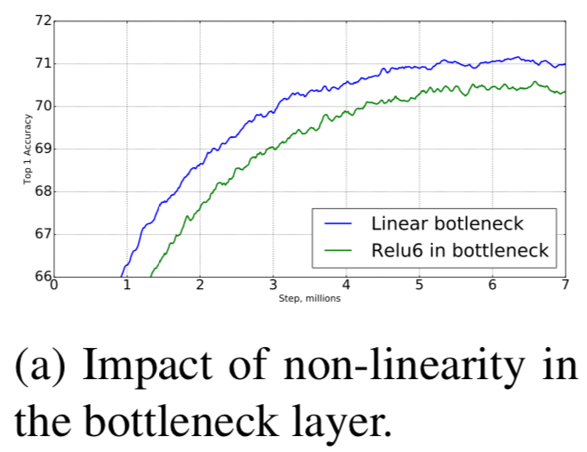
Importance of linear bottlenecks

• linear bottleneck model이 non-linearity model보다 더 적은 성능을 보인다.
  왜냐하면 activation들이 항상 linear regime에서 계산되어지기 때문이다.

• 하지만 Figure 6a에서 보여진 우리의 실험은 linear bottleneck이 performance를 향상시킨다고 보여준다.
  non-linearity가 low-dimensional space에 대한 정보를 파괴한다는 것을 보여준다.
  

---

7. Conclusions and future work

• 우리는 mobile model에 사용할 수 있는 매우 간단한 network architecture를 소개했다.
  우리의 basic bilding unit은 여러가지 properties를 갖는다.
  그것은 memory-efficient inference와 모든 neural frameworks에서 standard operation으로 사용되어지게 한다.

• 제안된 convolutional block은
  bottleneck input으로 encode된 capacity와 expansion layer로 encode된 expressiveness가 분리되어지는 것을 허용하는 독특한 property를 갖는다.
  이에 대해 탐구하는 것은 future research에서 중요한 방향이될 것이다.

---

My Conclusion

---

Seminar - Discussion

• "activation들이 subspace에 흩뿌려져 있는게 아니라 subspace에 모여있을 것이다."
  3차원 공간 안에 2차원 공간이 무수히 많이 있듯이, activation이 형성한 manifold of interest의 subspace에 고양이에 대한 feature들이 모여있을 것이다.
  이 또한 수학적 증명은 아니고 일종의 hypothesis이다..

• depthwise로 차원 정보가 깨지고
  projection을 해서 차원을 합치는 depthwise separable convolution은
  기존의 convolution 연산의 manifold 변환과는 다르다..

• 이론상 MobileNet의 parameter가 10배 정도 줄었으니 10배 빨라야 하는데, 실제로 그렇지 않다.
  NVIDIA에서 CNN을 위한 cuda programming 패키지인 dnn-utils를 제공하는데
  depthwise convolution에 대한 optimization을 구현해놓지 않았기 때문에
  이론상 runtime 시간과 실제의 runtime 시간의 차이가 있는 것이다..

• 연산량을 MAdds(Multiply Add)로 측정하는 논문, FLOPs(FLoating point Operations Per Second)로 측정하는 논문도 있고, ...,
  그래서 논문을 볼 때 이러한 차이점들에 대해서 유의하여야 한다.

• efficient network를 생각할 때, parameter size와 연산량을 분리하여 생각해야 한다.
  단순하게 추상적으로 efficient network의 size가 작다고 표현하면 안된다.
  efficient network를 설계할 때, parameter size를 줄일 것인지? 연산량을 줄일 것인지? 생각하고 그에 맞게 설계를 해야 한다.
  그리고 뭐가 작아진 것인지도 정확히 파악해야 한다.