[2016 CVPR] (ResNet) Deep Residual Learning for Image Recognition

Info
- authors : Kaiming He, Xiangyu Zhang, Shaoqing Ren, Jian Sun
- 학회 : Computer Vision and Pattern Recognition (cs.CV)
https://arxiv.org/abs/1512.03385
Abstract
-
Deeper neural network는 train시키기에 훨씬 어렵다.
우리는 이전에 사용되었던 것보다 더 사용하기 쉬운 residual learning framework를 소개한다.
우리는 layer의 input을 참조하는 residual function을 학습하는 layer를 reformulate시켰다. -
우리는 이 residual network가 optimize하기에 더욱 쉽고,
increased path에 상당히 높은 accuracy를 받을 수 있다는 것을
경험적인 evidence로 제공한다. -
The depth of representation은 많은 visual recognition task들에 매주 중요하다.
우리의 Deep residual net은 ILSVRC & COCO 2015 competition에 제출하였고,
그것은 ImageNet detection, ImageNet localization, COCO segmentation에서 1등을 했다.
1. Introduction
(Background: network depth는 image recognition에서 중요하다)
- Deep CNN은 image classification에 대한 breakthrough 중 하나로 여겨지고 있다.
Deep network는 자연스럽게 low/mid/high level features와 classifier에 있는 end-to-end multilayer fashion이 통합되고 있다.
최근 연구에서는 network depth가 매우 중요하다고 밝혀졌다.
그리고 ImageNet dataset에 대한 challeenging 결과들 모두 16~30 depth를 갖는 "very deep" model을 이용한다.
또 아직 밝혀지지 않은 많은 visual recognition tasks들 또한 very deep models로부터 굉장한 이득을 받고 있다.
(motivation)
- depth의 중요성에 기반하여, 한가지 궁금증이 떠오른다.
Is learning better networks as easy as stacking more layers?
(더 나은 network를 학습하는 것만큼 더 많은 layer를 쌓는게 쉬운가?)
이 질문에 대한 한가지 obstacle은 익히 알려진 vanishing/explolding gradients이다.
vanishing/exploding gradients는 convergence를 방해한다.
하지만 이 문제를 해결하기 위해 normalized initialization과 Batch normalization이
10개의 layer를 갖는 network의 converging을 가능하게 했다.
(이 논문의 문제 제기: plain network에서의 deeper network의 degradation 문제)
- deeper network가 converging을 시작하게 될 때,
degradationproblem에 노출된다.
degradation이란, depth increasing과 함께 accuracy가 saturated되고, 곧 이어 accuracy가 급격하게 하락하는 것을 의미한다.
뜻밖에도 degradation은 overfitting에 의해 발생하지 않으며,
더 많은 layer를 쌓는 것은 higher training error를 발생시킨다.
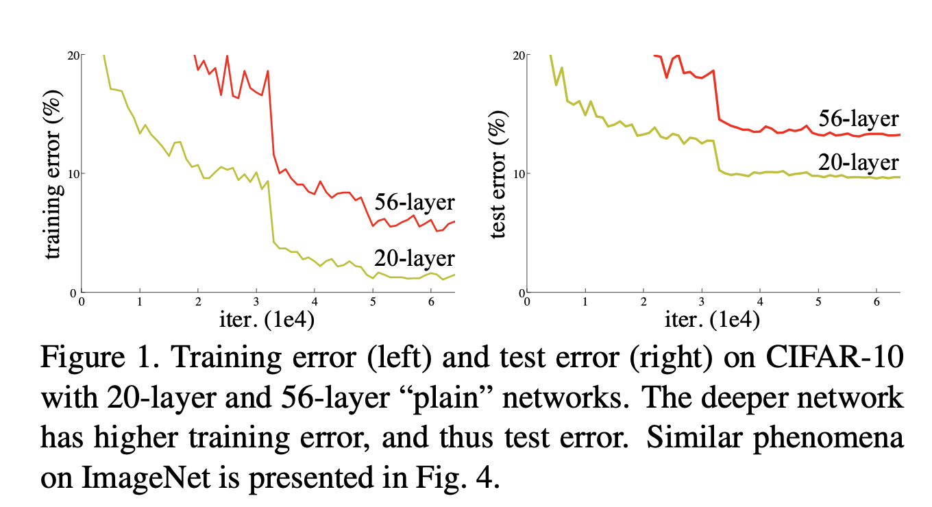
(아래 Fig.1에서 deeper=56-layer network의 training error와 test error가 동시에 높기 때문에 overfitting 현상은 아니고,
degradation 현상이라고 주장)

- degradation (of training accuracy)는 모든 system이 쉽게 optimize될 것이라고 보여지지 않는다.
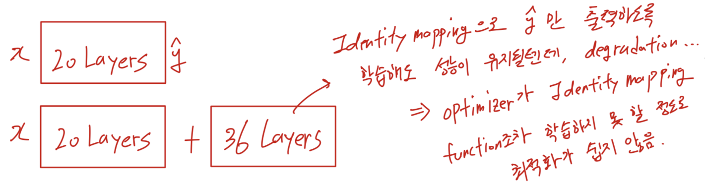
shallow architecture와 그에 대해 layer를 더 쌓은 deeper counterpart가 있다고 가정했을 때,
deeper model에 대해 construction에 의한 solution이 존재한다: 새로 추가된 layer에 대해서 shallow network가 만들었던 output을 그대로 Identity mapping하게 된다면,
이론적으로 deeper model은 shallower counterpart보다 똑같은 성능을 내거나 higher training error를 생성하지 않을 것이다.
하지만 우리의 실험 결과, deeper model의 optimization이 더 형편 없었다.
이것은 solver(optimizer)들이 deeper layer에서 아무것도 하지 않고 그대로 통과시키는 identity mapping조차 제대로 찾아내어 학습하지 못할 만큼 최적화 난이도가 높다는 것을 의미한다.
- degradation (of training accuracy)는 모든 system이 쉽게 optimize될 것이라고 보여지지 않는다.
-
degradation은 모든 system이 쉽게 optimize되지 않는다는 것을 보여준다.
우리는 이 논문에서,
deep residual learning framework를 소개함으로써 degradation problem을 해결할 것이다.
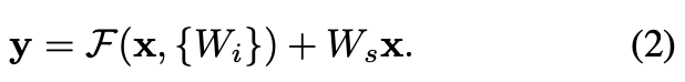
Formally,
우리가 원하는 기본적인 mapping을 라고 하고,
stacked nonlinear layer 가 mapping에 맞도록 하자.
그러면 original mapping은 로 recast된다.
우리는 기존의 unreferenced mapping(참조하지 않는)보다 residual mapping이
optimize하는 데에 더욱 쉬울 것이라는 가설을 세웠다.
공식은 "shortcut connections"을 갖는 feedforward neural network라고 생각할 수 있다.
Shortcut connection은 하나 이상의 layer를 skip하는 것이다.
우리의 경우, shortcut connection은 간단하게indentity mapping으로 구현했다.
전체 network는 기존 network의 수정 없이
여전히 end-to-end by SGD with backpropagation으로 train되어질 수 있다. -
ImageNet classification dataset에 대해서, 우리는 deep residual nets에 의해 훌륭한 결과를 얻었다.
Our 152-layer residual net is the deepest network ever presented on ImageNet, while still having lower complexity than VGG nets.
Our ensemble has 3.57% top-5 error on the ImageNet test set, and won the 1st place in the ILSVRC 2015 classification competition.
그리고 또 다른 recognition task들에 대해서도 놀라운 성능을 보여줬다.
(ImageNet detection, ImageNet localization, COCO detection, COCO segmentation에서도 1등)
이러한 성능을 통해 또 다른 vision 분야와 non-vision problem에 대해서도 적용가능할 것이라 기대되어진다.
2. Related Work
Residual Representations
- In image recognition, VLAD(Vector of Locally Aggregated Descriptors) is a representaion that encondes by the residual vectors with respect to a dictionary.
VLAD는 image retrieval과 classification에 대한 shallow representation에 강력하다.
low-level vision and computer graphics에서는 PDEs(Partial Differential Equations)을 풀기 위해,
널리 사용되는Multigrid method는 system을 multiple scales에서 subproblem으로 세분화하여,
각각의 subproblem이 coarser와 finer scale 사이의 reisudal solution 대해 책임감을 갖는다.(?)
➡️ VLAD, Multigrid 같은 methods는 optimization을 간략화할 수 있는 좋은 reformulation or preconditioning을 제안했다.
Shortcut Connections
-
shortcut connection은 오랫동안 연구되어져 왔다.
-
[34, 49] :
초기 MLPs 학습에 사용되었던 것은 network input에서 output으로 연결되는 linear layer를 추가하는 것이다. -
[44, 24] :
중간에 있는 layer들은 vanishing/exploding gradients를 해결하기 위해
직접적으로 auxiliary classifier와 연결되었었다. -
[39, 38, 31, 47] :
이 paper들은 centering layer responses, gradients, and propagated errors를 shortcut connection을 수행하여 제안했다. -
[44] :
"inception" layer는 shortcut branch와 few deeper branches로 구성되어졌다. -
우리의 연구와 비슷한 "highway networks"는 gating function으로 된 shortcut connection을 제시한다.
이 gates는 data-dependent하고 parameter를 갖는다.
반대로 우리의 identity shortcuts은 parameter를 갖지 않는다.
그리고 gated shortcut이 "closed(approaching zero)"될 때,
highway network의 layer들은 non-residual function을 표현한다.
하지만 우리의 formulation은 항상 residual function을 학습한다
우리의 identity shortcut은 절대 closed되지 않고, 모든 정보는 항상 통과해간다.
또한 high-way network는 increased depth에 대한 accuracy를 증명하지 않았다.
3. Deep Residual Learning
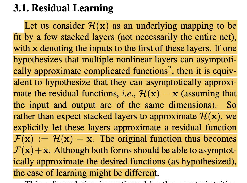
3.1 Residual Learning
-
a few stacked layer를 mapping시키는 가 있다고 가정하자.
(는 이 layer들의 첫번째 input이다)
만약 multiple nonlinear layer들이 점진적으로 complicated function을 approximate한다고 가정하면,
그것들은 점진적으로 residual function ()를 approximate한다는 것과 같다.
그래서 를 근사하는 layer를 쌓는 것 대시에,
우리는 명시적으로 이 layer들이 residual function()에 근사하도록 할 것이다.
그러므로 original function은 가 된다.
비록 두 함수는 desired function에 근사할 수 있지만, learning의 용이성이 다르다. -
이 reformulation은 degradation problem에 대해 직관에 반하여 동기가 되었다.
만약 추가된 layer들이 identity mapping을 구성할 경우,
deeper model은 shallower model보다 더 크지 않는 training error를 가져야 한다.
실제 경우에는 identity mapping이 optimal이라고 보기 쉽지는 않지만
our reformulation은 그 문제를 precondition하는 데에 도움이 될 것이다.
만약 optimal function이 identity mapping과 가깝다면,
solver가 identity mapping을 참조하여 혼란(perturbation = 미세한 조정)을 찾기에 쉬울 것이다.
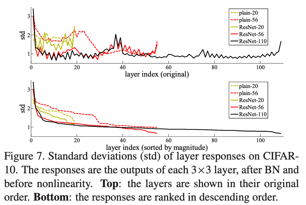
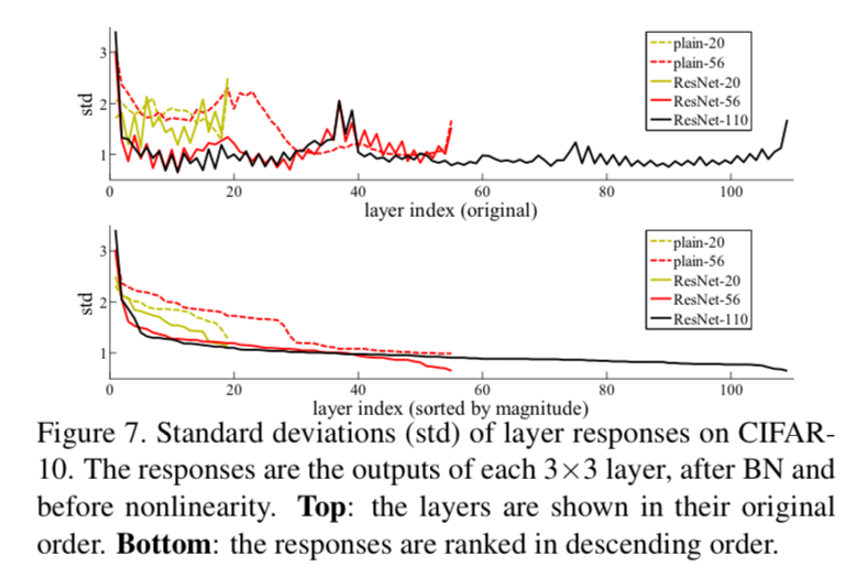
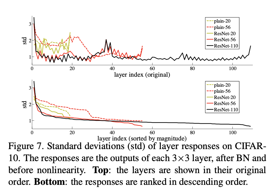
우리는 Figure7에서 learned residual function이 small response를 갖는다는 것을 실험적으로 보여줬고
identity mapping이 reasonable preconditioning이라는 것을 제시한다.- 시간이 지나 (2026.03.26) ResNet을 다시 읽고 해석:
network가 깊어질수록 대부분의 layer는 원본 입력을 크게 변형하지 않고 아주 미세한 조정(perturbation)만 수행한다는 것을 시각적으로 증명한 그래프.
각 layer를 통과한 출력값의 standard deviation을 나타냄.
ResNet 구조에서, shortcut을 제외한 실제 의 크기를 측정한 것.
이게 왜 중요하냐면? 만약 optimal function이 zero mapping보다 Identity mapping에 가깝다면,
새로운 함수를 처음부터 배우는 것보다 indentity function을 기준으로 작은 변화 (Perturbation)만 찾는 것이 solver에게 훨씬 쉬울 것이라는 가설을 간접적으로 뒷받침할 수 있기 때문.
즉, 수많은 layer들이 복잡한 변환을 억지로 학습하느라 고생하는게 아니라, 기본적으로 이전 layer의 정보 를 그대로 identitiy mapping으로 흘려보내면서, 아주 살짝만 값을 보정()하는 역할을 하고 있다는 뜻.
- 시간이 지나 (2026.03.26) ResNet을 다시 읽고 해석:
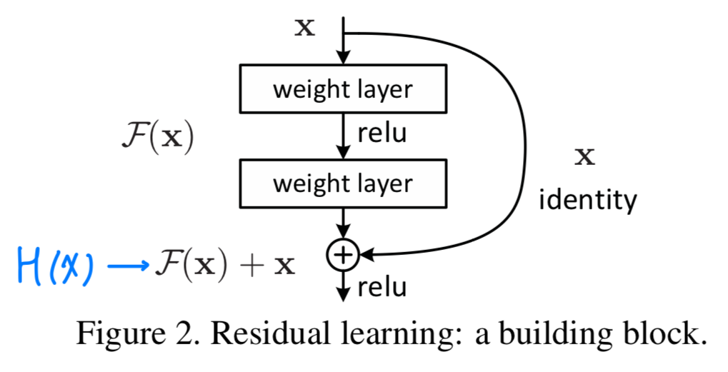
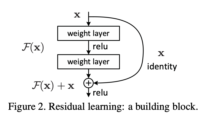
3.2 Identity Mapping by Shortcuts
- 우리는 every few stacked layer에 residual learning을 적용했다.
a building blockis shown in Fig.2.
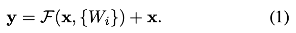
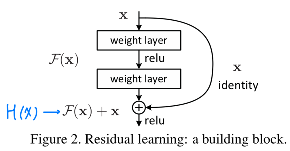 공식적으로, 이 논문에서 우리는 buliding block을 다음과 같이 정의했다.
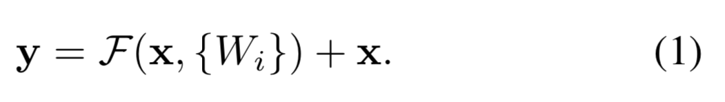 (와 는 layer의 input과 output vector이다.)
는 학습되어진 residual mapping을 나타낸다.
Figure 2에서는 두 개의 layer를 갖는다
in whicn denotes ReLU and the biases are omitted for simplifying notations.
is performed by a shortcut connection and element-wise addition.
우리는 두번째 nonlinearity를 addition 이후에 적용했다. Figure 2에서 .
Eqn.(1)에서 shortcut connection은 extra parameter나 computation complexity를 포함하지 않는다.
우리는 공평하게 plain/residual network를 동시에 같은 parameter수, depth, width, computational cost로 비교할 수 있다.
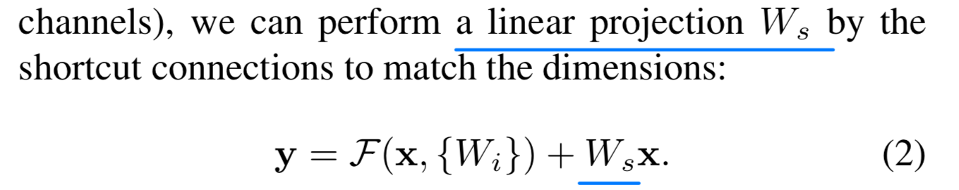
Eqn.(1)에서 와 의 dimension이 같아야 한다.
만약 다르다면, 우리는 dimension을 일치시키기 위해 linear projection 를 수행할 수 있다.
우리는 또한 Eqn.(1)에서 square matrix 를 사용할 수 있다.
하지만 실험에서 확인한 결과, 는 matching dimension할 때만 유용하다는 것을 알 수 있다.
 residual function 의 형태는 유동적이다.
이 논문의 Experiments에서 2개 또는 3개 layer를 갖는 function 를 포함했지만, 더 많은 layer를 포함할 수도 있다.
하지만 가 single layer라면, Eqn.(1)은 linear layer와 비슷하다. ()
우리는 이러한 residual function에 대한 이점을 발견하지 못했다.
우리는 또한 위 notation들을 편의를 위해 FC layer로 했어도, convolutional layer에도 적용이 가능하다.
function 가 multiple conv layer를 나타낼 수 있다.
element-wsie addition은 채널별로 두 feature map에서 수행된다.
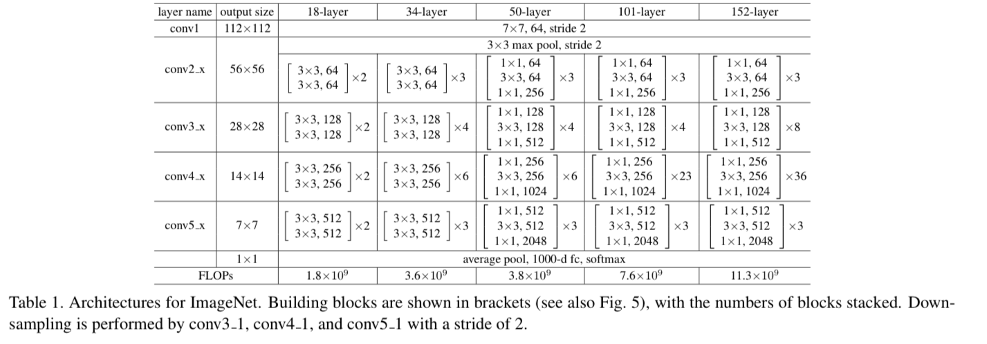
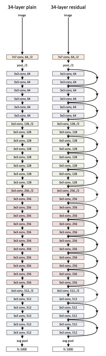
3.3 Network Architecture
- 우리는 다양한 plain/residual net을 test해왔다.
discussion할 거리를 제공하기 위해 ImageNet에 대한 두가지 model은 다음과 같다.
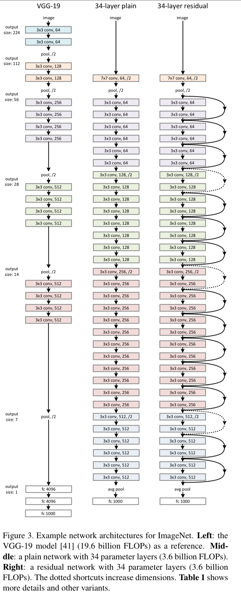
Plain Network
- 우리의 plain baseline은 주로 VGGnet의 철학에서 영감을 받았다.
convolutional layer는 3x3 filter를 갖고 2가지 간단한 rule을 따른다.- 똑같은 output feature map에 대해서, 해당 layer는 똑같은 filter 개수를 갖는다.
- 만약 feature map size가 절반이 되었다면, filter의 개수를 2배로 한다.
- 우리는 stride=2인 conv layer로 downsampling을 수행한다.
network는 global average pooling layer로 끝나고 1000-way FC layer with softmax를 갖는다.
wegithed layer의 최종 개수는 34개이다. (Fig 3)
It is worth noticing that our model has fewer filters and lower complexity than VGG nets.
Our 34-layer baseline has 3.6 billion FLOPs(multiply-adds),
which is only 18% of VGG-19 (19.6 billion FLOPs)
Residual Network
- 위 plain network에 기반하여, 우리는 shortcut connection을 insert했다.
- The identity shortcuts (Eqn.(1)) cab be directly used
when the input and output are of the same dimensions(solid line shortcutsin Fig. 3).
dimension이 증가할 때(dotted line shortcutsin Fig.3), 우리는 2가지 옵션을 고려한다- A :
The shortcut still identity mapping, with extra zero entries padded for increasing dimensions.
(identity mapping이지만, 차원을 늘려주기 위해 0로 padding)
This option introduces no extra parameter - B :
The projection shortcut() in Eqn.(2) is used to match dimensions
(done by 1x1 convolutions).
➡️ for both options, when the shortcuts go across feature maps of two sizes,
they are performed with a stride of 2.
- A :
3.4 Implementation
-
image is resized with its shorter side randomly sampled in [256, 480] for scale augmentation.
-
A 224x224 crop is randomly sampled from an image or its horizontal flip, with the per-pixel mean subtracted. (21:AlexNet)
-
The standard color augmentation in [21] is used.
-
We addopt BN(16) right after each convolution and before activations.
-
we initialize the weights as in 13 and train al plain/residual nets from scratch.
-
We use SGD with a mini-batch size of 256.
-
The learning rate starts from 0.1 and is divided by 10 when the error plateaus,
and the models are trained for up to 600,000 iterations.
We use a weight decay of 0.0001 and a momentum of 0.9. -
We do not use dropout.
-
In testing, for comparison studies we adopt the standard 10-crop testing.
For best results, we adopt the fully-convolutional form as in [41, 13],
and average the scores at multiple scales(images are resized such that the shorter side is in {224, 256, 384, 480, 640}).
4. Experiments
4.1 ImageNet Classification
- We evaluate our method on the ImageNet 2012 classification dataset that consists of 1000 classes.
(1.28 millilon training images, and evaluated on the 50k validation images)
We also obtain a final result on the 100k test images.
Plain Networks
- We first evaluate 18-layer and 34-layer plain nets.
The 34-layer plain net is in Fig. 3(middle).
The 18-layer plain net is of a similar form.
See Table 1 for detailed architectures.
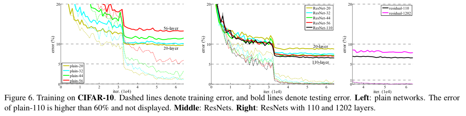
- The results in Table 2 show that the deeper 34-layer plain net
has higher validation error than the shallower 18-layer plain net.
To reveal the reasons, in Fig.4 (left)
we compare their training/validation errors during the training procedure.
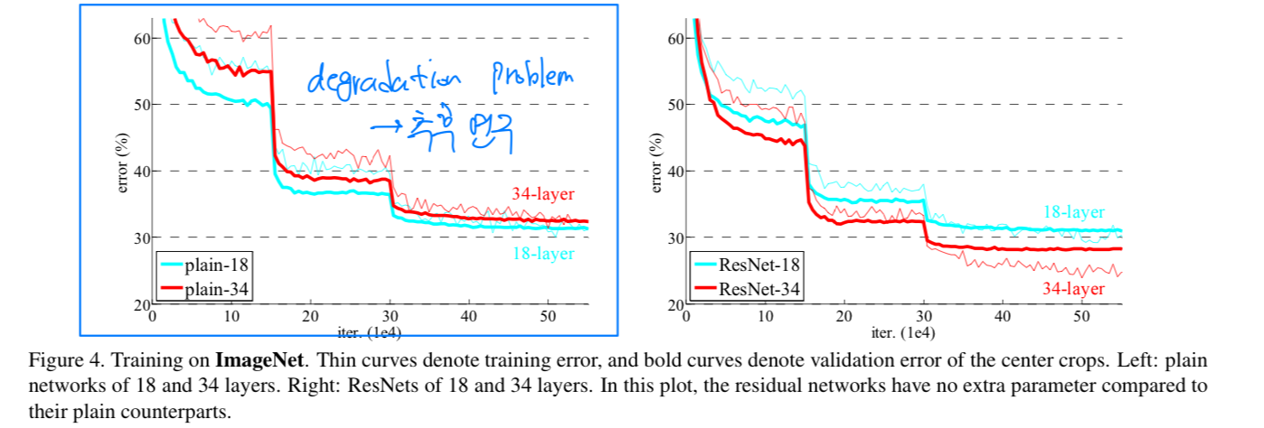
We have observed the degradation problem -
the 34 layer plain net has higher training error throughout the whole training procedure,
even though the solution space of the 18 layer plain network is a subspace of that of the 34 layer one.
우리는 이 optimization difficulty를 vanishing gradient로 인해 발생한 것이라고 보기 어렵다고 주장한다.
이 plain network들은 BN에 의해 train되어 졌고, propagated signal이 non-zero variance를 갖도록 보장되어진다.
우리는 또한 backward propagated gradient가 BN과 함께 건강한 norms을 나타낸다고 확인했다.
그래서 forward나 backward signal vanish 문제가 아니다.
사실, 34-layer plain net은 여전히 competitive accuracy를 달성할 수 있다.
우리는 deep plain nets이 exponentially low convergence rate를 가질 수 있다고 추측하고,
그것은 training error를 줄이는 데에 해가 된다고 추측한다.
이 optimization difficulty에 대한 이유는 추후에 연구되어질 것이다.
정리) deeper plain net에서 degradation 문제의 원인은 잘 모르겠고, 추후 연구할 것임 (?)
Residual Networks
-
we evaluate 18-layer and 34-layer residual nets.
baseline architecture는 plain net과 똑같고, shortcut connection이 각 3x3 filter에 더해졌다.
Fig. 3 (right) -
In the first comparison (Table 2 and Fig.4 right),
we use identity mapping for all shortcuts and zero-padding for increasing dimensions.
So they have no extra parameter compared to the plain counterparts.
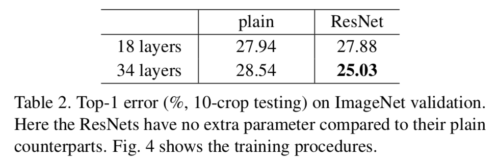
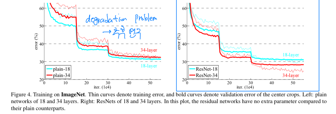 We have 3 major observations from Table 2 and Fig.4.
- this situation is reversed with residual learning - the 34-layer ResNet is better than the 18-layer ResNet.
This indicates that the degradation problem is well addressed in this setting and we manage to obtain accuracy gains from increased depth. - compared to its plain counterpart, the 34-layer ResNet reduces the top-1 error by 3.5%, resulting from the successfully reduced training error.
This comparison verifies the deffectiveness of residual learning on extremely deep systems. - we also note that the 18-layer plain/residual nets are comparably accurate,
but the 18-layer ResNet converges faster.
When the net is "no overly deep"(=18-layer), the current SGD solver is still able to find good solutions to the plain net.
- this situation is reversed with residual learning - the 34-layer ResNet is better than the 18-layer ResNet.
Identity vs Projection Shortcuts
- We have shown that parameter-free,
identity shortcutshelp with training.
Next we investigateprojection shortcuts(Eqn.(2))
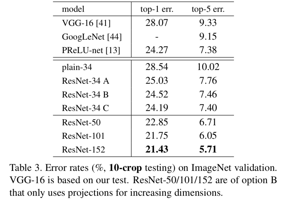 In Table 3 we compare 3 options :
 - (A) :
zero-padding shortcuts are used for increasing dimensions,
and all shortcuts are parameter-free - (B) :
projection shortcuts are used for increasing dimensions,
and other shortcuts are identity - (C) :
all shortcuts are projections.
Table 3는 모든 3가지 옵션이 plain counterpart보다 낫다는 것을 보여준다.
B는 A보다 조금 더 낫다.
우리는 이 이유를 A에서 zero-padded dimension들은 실제로 residual learning이 필요없기 때문이라고 주장한다.
C는 부분적으로 B보다 낫다.
그리고 우리는 많은(13-layer) projection shortcut에 의한 추가적인 parameter에 영향을 받았다고 생각한다.
하지만 A/B/C 사이에서 아주 작은 차이점이 있다.
그것은 projection shortcut이 degradation problem을 해결하는 데에 필수적이지 않다는 것이다.
그래서 우리는 memory/time complexity와 model size를 줄이기 위해,
이 논문의 나머지에서도 option C를 사용하지 않았다.
Identity shortcuts은 다음으로 소개할 bottleneck architecture의 complexity를 증가하지 않기 위해 중요하다.
- (A) :
Deeper Bottleneck Architecture
- 다음으로 우리는 ImageNet을 위한 deeper net을 설명하겠다.
우리가 사용할 수 있는 training time에 대한 우려로 인해,
우리는 building block을 bottleneck design으로 수정했다.
각 residual function 에,
우리는 2개의 layer 대신 3개의 layer를 쌓았다.
3개의 layer는 1x1, 3x3, 1x1 convolution이고, 1x1 layer는 dimesion을 줄이고 늘리는 데 사용된다.
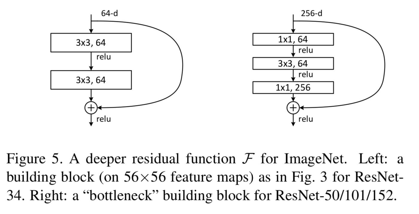
헷갈렸던 내용 :
projection option C 에서 1x1 convolution을 하지 않는다는 것과
bottleneck architecture의 layer에 1x1 convolution을 적용한다는 것은
완전히 다른 내용임.
projection option C 에서 1x1 convolution을 하지 않는다는 것 :
를 곱해줘서 차원이 증가하는 것을 맞춰주기 위해 projection을 할 때, 1x1 convolution을 사용하겠다는 것임.
이는 memory/time complexity가 늘어나기 때문에 이 논문에서 고려하지 않았음
bottleneck architecture의 layer에 1x1 convolution을 적용한다는 것 :
computational cost를 줄이기 위해 기존 3x3 conv layer를 1x1 3x3 1x1 conv layer로 바꾼 것임.
50-layer ResNet
- 우리는 34-layer net의 2-layer를 3-layer bottleneck block으로 교체했고,
resulting in a 50-layer ResNet (Table 1).
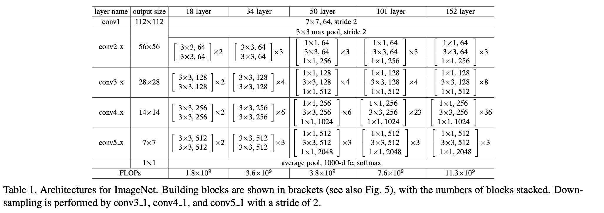
101-layer and 152-layer ResNets
-
우리는 더 많은 3-layer blocks을 이용하여 101-layer와 152 layer를 만들었다.
놀랍게도 depth가 증가했음에도 152-layer ResNet이 여전히 lower complexity than VGG-16/19. -
The 50/101/152-layer ResNet은 34-layer보다 훨씬 더 정확하다.
우리는 degradation problem을 관찰하지 않았고 increased depth로부터 significant accuracy을 얻었다.
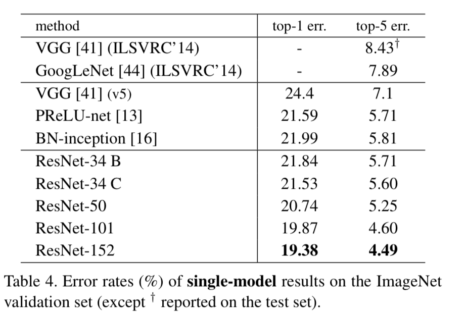
Comparison with State-of-the-art Methods
- In Table 4,
we compare with the previous best single-model results.
4.2 CIFAR-10 and Analysis
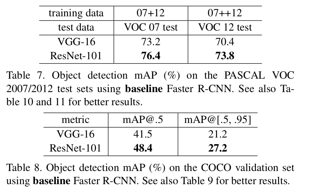
4.3 Object Detection on PASCAL and MS COCO
Seminar - discussion
- 이 논문은 residual block을 사용해서 ILSVRC 2015에서 1위를 한 architecture를 소개하였지만,
conjecture이 너무 많아서 좋은 논문이라고 보기에는 어렵다.- degradation이 왜 발생하는가?
이 논문에서는 추후에 연구로 남겨둔다고 했다. (= 모른다고 했다)
우선 이 논문에서 plain network의 depth가 증가할수록 training, test error가 높아진다는 실험적 예시를 보여줬다
논문에서는 training error와 test error 둘 다에 degradation 현상이 발생했기 때문에
overfitting 문제라고 주장하지 않았다.
또한 논문에서는 BN을 사용했기 때문에 gradient vanishing/exploding 문제도 발생하지 않을 것이라고 주장했다.내 생각 :
확실치는 않지만 BN을 적용했더라도 vanishing문제가 발생하지 않을까?
BN을 적용했더라도 depth가 늘어날수록 gradient signal이 작아져서 끝까지 도달하지 못할 것이라고 생각한다
plain network(34-layer plain)가 residual network보다 성능이 안좋은 이유도 이와 같을 것이다.
residual network(34-layer residual)는 중간에 shortcut connection을 통해 gradient signal이 pumping되어 끝까지 도달하는 데에 도움이 될 것이다.
- degradation이 왜 발생하는가?
- 논문에서 궁금증을 가졌던 부분 :
 이 부분에 대해서 완전한 이해가 되지 않았었다.
는 우리가 원하는 mapping이고 Fig2. 를 봤을 때, 의 형태이기 때문에
위 글에서 왜 라고 적어놨는지 이해가 되지 않았다.
알고보니 저자의 의도는 다음과 같다.
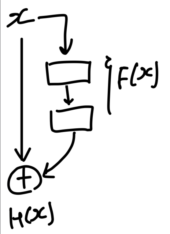 이전 layer에서 전달되는 x는 고정되어 있고, 우리는 해당 residual block에서 만 학습하면 되는 것이다.
따라서 Residual block의 Residual의 의미는 "잔차, 나머지"이므로
라는 잔여의 학습할 양을 의미한 것이었다.
만약 mapping이 없었다면, F(x)+x 를 모두 학습했어야 했지만
mapping을 연결해줌으로 인해, F(x)만 학습하면 되는 것이다.
다음 layer에서 학습할 양을 덜어준다.
는 중심의 값이 되고, residual block에서는 만 학습하면 된다.
이처럼 모든 block은 자신의 해당하는 F(x)만 학습하면 되는 것이다.
논문 마지막 쯤에 BN과 같이 std deviation이 작고, 일정하게 유지되는 효과를 언급했다.
 아마 잔여된 학습 의 효과가 BN의 효과와 비슷한 것 같기 때문이다.
BN도 비슷하게 covariate shift(밑에서 바뀌면 뒤에도 다 바뀌었는데)로 학습이 어려워서,
각 Layer의 input을 normalization시켜서 std deviation을 일정하게 유지시켜줬었다.
ResNet도 비슷하게 이전 layer의 output인 x가 계속 바뀌면 뒤에서 바꿔야 할 값들도 바뀌기 때문에,
x를 고정한 채로 residual block에서 F(x)만 학습시키도록 하여 효과적으로 학습시키는 효과를 낼 수 있다.
그래서 잔여학습 = 잔여된 F(x)를 학습하는 block을 계속해서 쌓음
