Computer vision

• Computer vision is one of the areas that's been advancing rapidly thanks to deep learning.

• Here are some exampels of computer vision problems we'll study in this course.
  You've already seen image classifications, sometimes also called image recognition,
  where you might take as input say a $64 * 64$ image and try to figure out is that a cat?
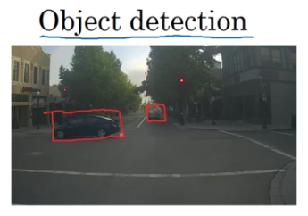  Another example of the computer vision problem is object detection.
  So if you're building a self-driving car,
  maybe you don't just need to figure out that there are other cars in this image.
  But instead, you need to figure out the position of the other cars in this picture,
  so that your car can avoid them.
  In object detection, usually we have to not only just figure out that these other objects say cars and pictures,
  but also draw boxes around them.
  And in this example, they can be multiple cars in the same picture,
  or at least every one of them with in a certain distance of your car.
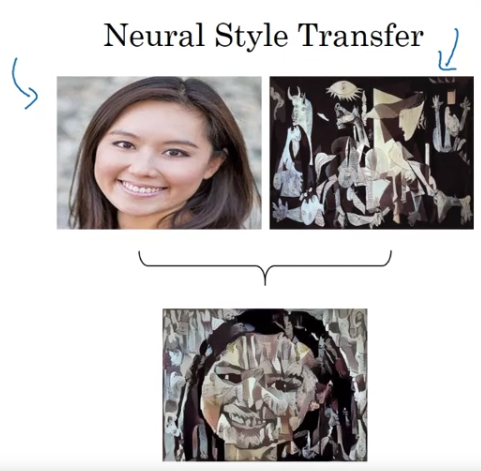  Here's another example, Neural Style Tranfer.
  Let's say you have a picture, and you want this picture repainted in a different style.

So Nueral Style Transfer,
you have a content image, and you have stlye image.
The image on the right is actually a Picasso.
And you can have a neural network put them together to repaint the content image.
So, algorithms like these are enabling new types of artwork to be created.

Deep Learning on large images

• One of the challenges of computer vision problems is that the inputs can get really big.
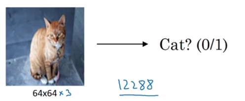  For example, in previous courses, you've worked with $64 * 64$ images.
  And so that's $64 * 64 * 3$ because there are three color channels.
  And if you multiply that outm that's $12288$.
  So $x$ the input features has dimension $12288$.
  And that's not too bad.
  $64 * 64$ is actually a very small image.
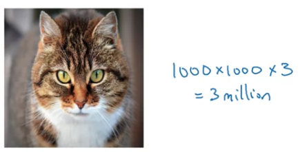  If you work with larger imgaes, maybe this is a $1000 * 1000$ image.
  The dimension of the input features will be $1000 * 1000 * 3$ because you have three RGB channels, and that's 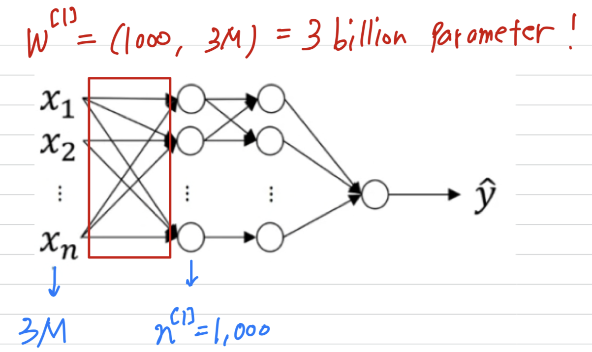$3 millilon$.Then this means that $X$ will be $3$ $millilon$ dimesnional.
  And so, if in the first hidden layer maybe you just a $10,000$ hidden units,
  then the total number of weights that is the matrix $W^{[1]}$ will have
  $3$ $billion$(30억) parameters which is just very, very large.
  And with that many parameters,

  it's difficult to get enough data to prevent a neural network from overfitting.
  And also, the computational memory requirements to train a neural network with $3$ $billon$ parameters is just a bit infeasible.
  
  But for computer visioon applications, you don't want to be stuck using only tiny little imgaes.
  You want to use large images.
  To do that, you need to better implement the convolution operation,
  which is one of the fundamental building blocks of convolutional neural networks.
  
  크기가 큰 input image를 학습하려면, neural network로는 힘들다

---

Edge Detection Example

• The convolution operations is one of the fundamental building blocks of a convolutional neurla network.
  Using edge detection as the motivating example.
  In this video you will see how the convolutional operation works.

Computer Vision Problem

• In previous video,
  I have talked about how the early layers of the neural network might detect edges
  and then the some later layers might detect cause of objects
  and then even later layers may detect cause of complete objects like people's faces in this case.
  In this video, you see how you can detect edges in an image.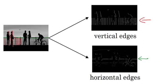Let's take an example.
  Given a picture like that for a computer to figure out what are the objects in this picture.
  The first thing you might do is maybe detect vertical edges in this image.
  And you might also want to detect horizontal edges.
  
  So how do you detect edges in image like this?

Vertical edge detection

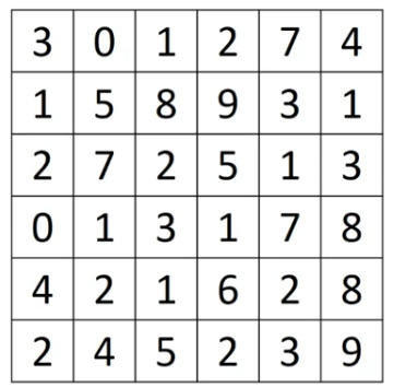• Here is a $6 * 6$ grayscale image.
  Because this is a grayscale image this is just a $6 * 6 * 1$ matrix.
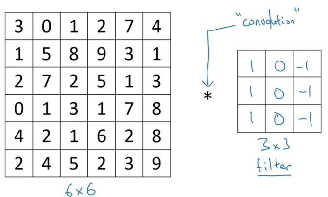  In order to detect edges or lets say vertical edges in this image,
  what you can do is construct a $3 * 3$ matrix
  and in the pollens when the terminology of convolutional neural networks,
  this is going to be called a filter.
  (Sometimes research papers will call a kernal instead of afilter but i am going to use the filter terminology in these videos.)
  And what you are gonna to do is take the $6 * 6$ image and convolve it with the $3 * 3$ filter.
  (수학에서의 $* =asterisk =별표$ 는 convolution symbol이지만,
  python에서의 $*$은 multiplication or element-wise multiplication symbol로 사용된다.)
  (이 강의에서는 asterisk($*$)를 convolution으로 나타낸다.)
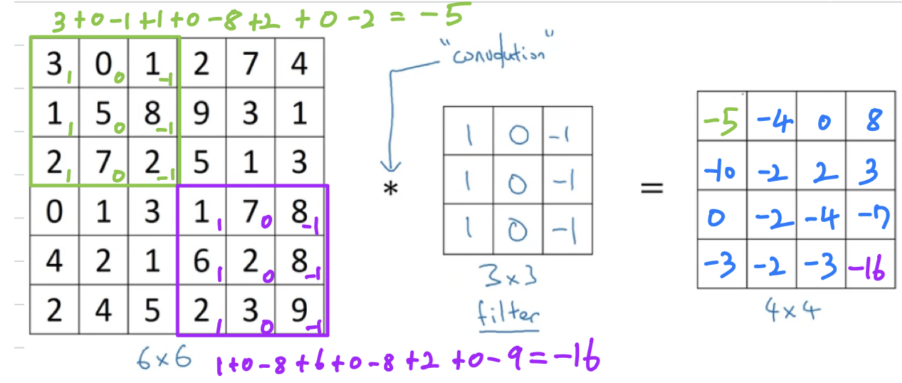  The output of this convolution operator will be $4 * 4$ matrix, which you can think of as a $4 * 4$ image.
  If you implement this in a programming language, some different functions rather than an asterisk to denote convolution.
  
  Why is this doing vertical edge detection?
  Let's look at another example.

• To illustrate this, we are goint to use a simplified image.
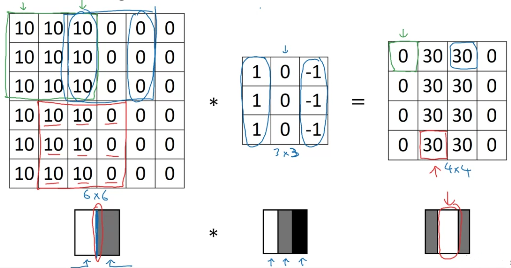  So here is a simple $6 * 6$ image.
  If you plot this as a picture, it might look like this
  where the left half, the $10$s give you brighter pixel intensive values
  and the right half, the $0$s give you darker pixel intensive values.
  (10과 0은 실제로 저런 색이 아니겠지만 예시를 위해 극단적으로 생각.)
  In this image, there is clearly a very strong vertical edge right down the middle of this image
  as it transitions from white to black color.
  
  So when you convolve this with the $3 * 3$ filter and so this $3 * 3$ filter can be visualized as follows,
  brighter pixels on the left
  and then mid tone zeroes in the middle
  and then darker on the right.
  
  In case the dimensions here seem a little bit wrong that the detected edges seems really thick,
  That's only because we are working with very small images in this example.
  And if you are using, say a $1000 * 1000$ image rather than a $6 * 6$ image then
  you find that this does a pretty good job(detecting the vertical edges in your image).

---

More Edge Detection

• You've seen how the convolution operation allows you to implement a vertical edge detector.
  In this video, you'll learn the difference between positive and negative edges,
  that is the difference between light to dark versus dark to light edge transitions.
  And you'll also see other types of edge detectors,
  as well as how to have an algorithm learn rather than have us hand code an edge detector.

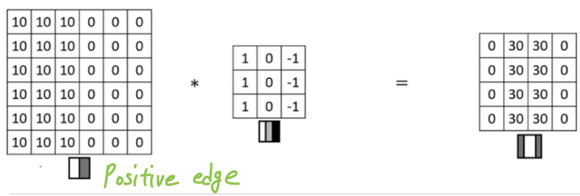• Here's the example you saw from the previous video,
  where you have this image $6 * 6$, there's light on the left and dark on the right.
  
  What happens in an image where the colors are flipped,
  where it is darker on the left and brighter on the right?
  If you convolve it with the same edge detection filter, you end up with $-30$s instead of $+30$s.
  전환되는 명함이 반대로 되기 때문에,
  기존에 밝은 색에서 어두운 색으로 바뀌는 것이 아니라 어두운 색에서 밝은 색으로 바뀌는 것임을 볼 수 있다.
  만약 위 두가지 경우 중 어느 것인지 상관이 없다면 output matrix에 절대값을 취할 수 있다.
  하지만 이 위 특정 filter는 밝은 색에서 어두운 색으로 변하는 edge와 어두운 색에서 밝은 색으로 변하는 edge의 차이점을 알 수 있다.

Vertical and Horizontal Edge Detection

• Let's see some more examples of edge detection.
  So here's one example.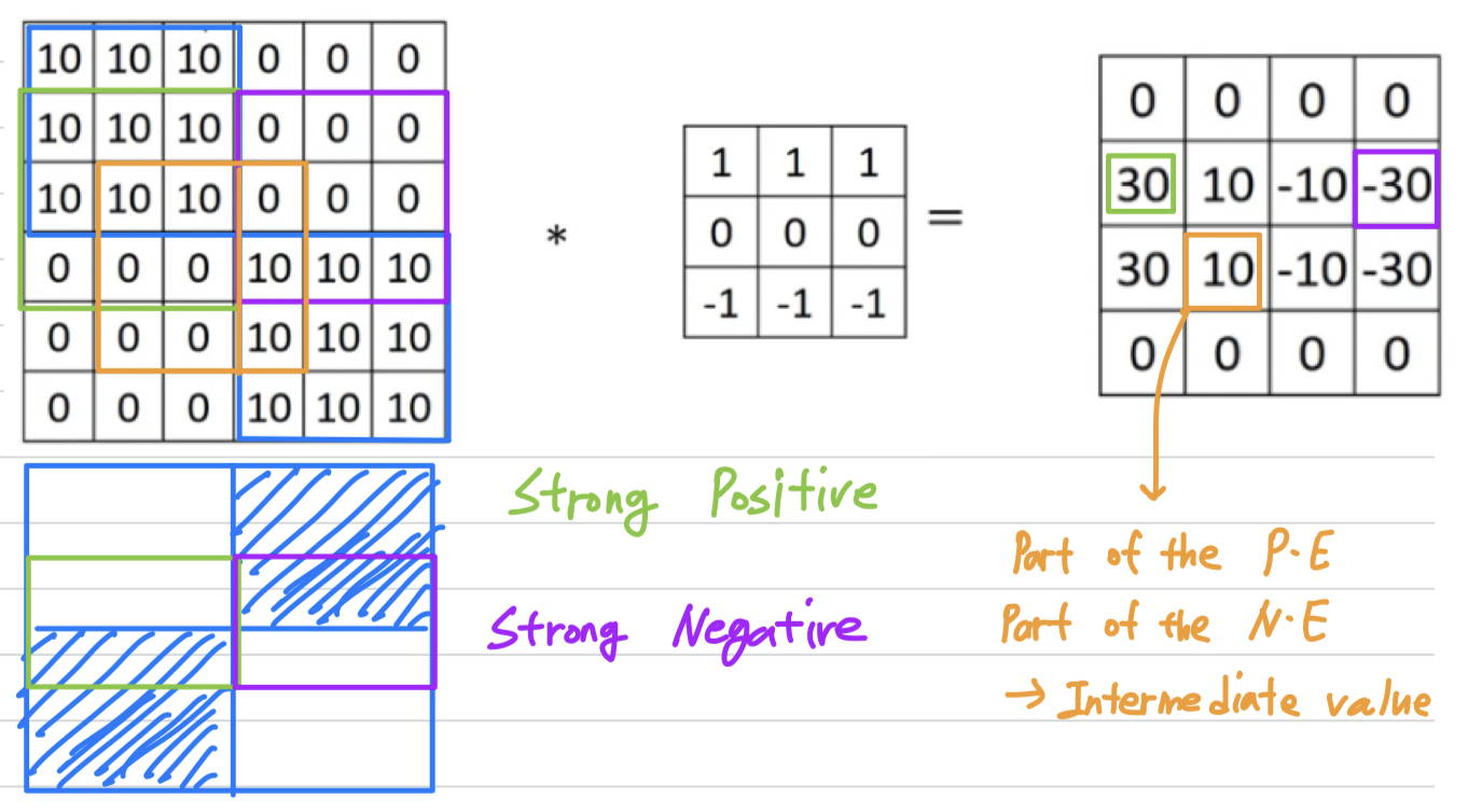If you convolve this with a horizontal edge detector, you end up with this.
  
  So in summary, different filters allow you to find vertical and horizontal edges.

  Learning to detect edges

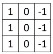• It turns out that the $3 * 3$ vertical edge detection filter we've used is just one possible choice.
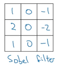  And historically, in the computer vision literature,
  there was a fair amount of debate about what is the best set of numbers to use.
  This is called a Sobel filter.
  And the advantage of this is it puts a little bit weight to the central row,
  and this makes it maybe a little bit more robust.
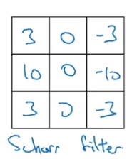  But computer vision researchers will use other sets of numbers as well.
  And this is called a Scharr filter.

• With the rise of deep learning,
  one of the things we learned is that
  when you really want to detect edges in some complicated image, maybe you don't need to have computer vision researchers handpick these nine numbers.
  Maybe you can just learn them and treat nine numbers of this matrix as parameters,
  which you can then learning using back propagation.
  
  And what you see in later videos is that by just treating these nine numbers as parameters,
  the backprop can choose to learn something else that's even better at capturing the statistics of you data than any of these hand coded filters(Sobel, Scharr).
  
  And rather than just vertical and horizontal edges,
  maybe it can learn to detect edges that are $45\degree, 70\degree, 73\degree, ...$ at whatever orientation it chooses.

---

Padding

• In order to build deep neural networks,
  one modification to the basic convolutional operation that you need to really use is padding.
  
• Let's see how it works.
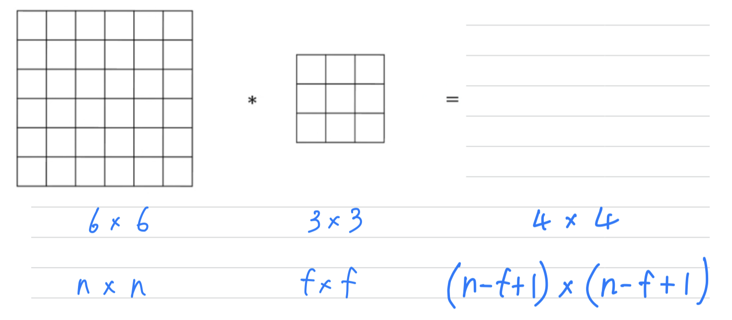  What we saw in earlier videos is that if you take a $6 * 6$ image and convolve it with a $3 * 3$ filter,
  you end up with a $4 * 4$ matrix ouptut.
  왜냐하면 $3 * 3$ filter가 $6 * 6$ matrix에 들어갈 수 있는 위치의 수는 $4 * 4$ 밖에 없기 때문이다.
  
  So the two downsides to this
  1. If every time you apply a convolutional operator, your image shrinks,
     so you come from $6 * 6$ to $4 * 4$.
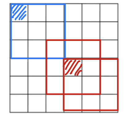
     Then you can only do this a few times before your image starts getting really small, maybe it shrinks down to $1 * 1$ or something.
  2. If you look the pixel at the corner or the edge, this little pixel is touched as used only in one of the outputs, because this touches that $3 * 3$ region.
     Whereas, if you take a pixel in the middle, then there are a lot of $3 * 3$ regions that overlap that pixel.
     따라서 모서리나 가장자리의 pixel들은 convolution 계산에 훨씬 적게 사용되어 많은 정보가 버려진다.
     
• To solve both of these problems(1. the shrinking output, 2. throwing away information from the edges of the image),
  what you can do is the full apply of convolutional operation.
  You can pad the image.
  
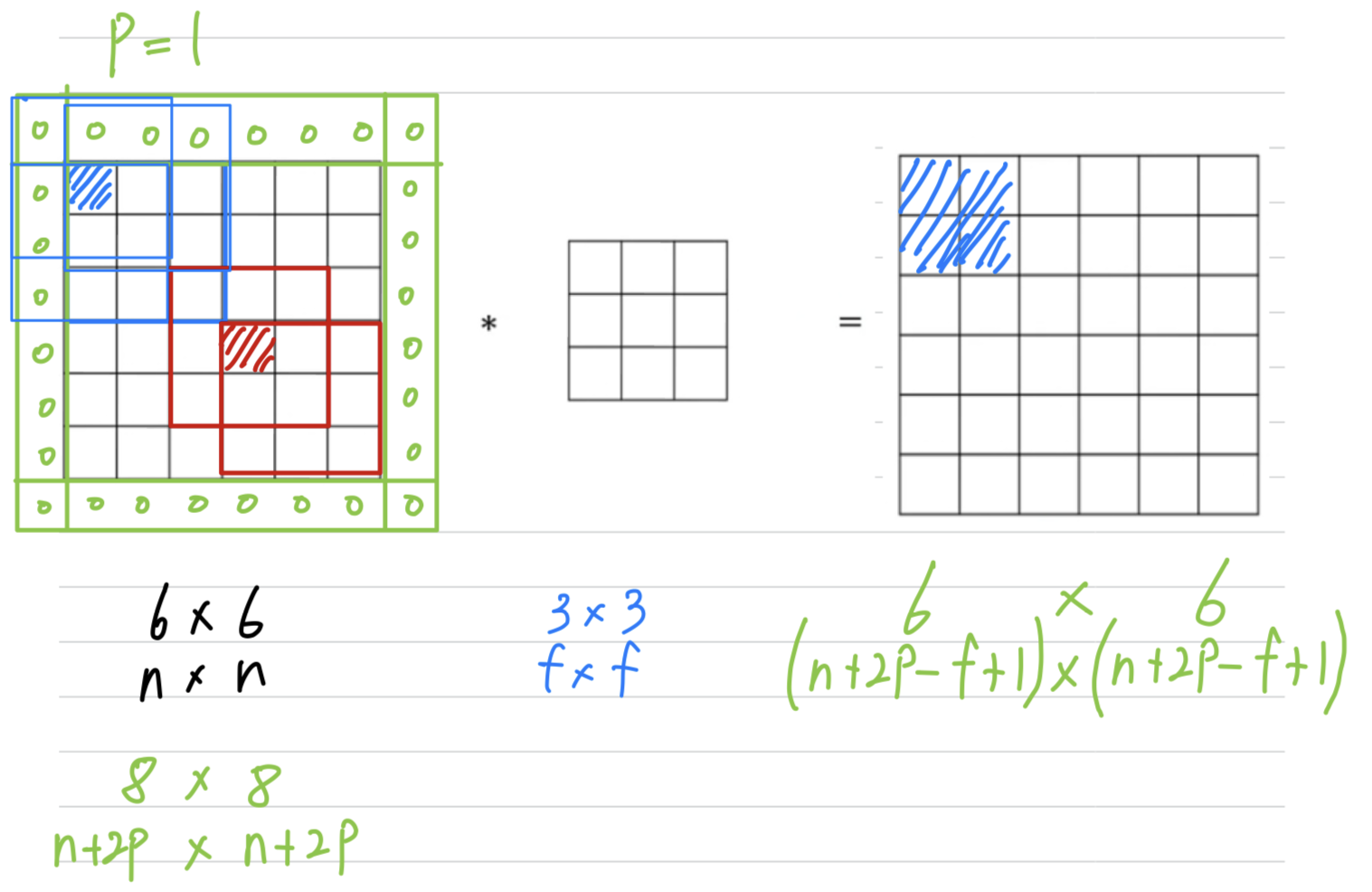
  so you managed to preserve the original input size of $6 * 6$.
  So by convention when you pad,
  you padded with zeros and if $p$ is the padding amounts.
  So you end up with a $6 * 6$ image taht preserves the size of the original imgae.
  
  So this being pixel actually influences all of these cells of the output.
  So this effect maybe not by throwing away but counting less the information from the edge of corner or the edge of the image is reduced.
  (출력의 모든 셀에 영향을 미치기 때문에 이미지의 모서리나 엣지의 정보를 버리지 않는 것으로 효과적임.)
  
  If you want, you can also pad the border with $2$ pixels. ($p=2$)

Valid and Same convolutions

• In terms of how much of pad,
  it turns out two common choices that are called, Valid convolutions and Same convolutions.
  1. Valid convolutions : No padding.
     $(n$ x $n)$ $*$ $(f$ x $f) = (n-f+1)$ x $(n-f+1)$
  2. Same convolutions : Pad so that output size is the same as the input size.
     (출력 크기가 입력 크기와 같도록 padding)
     when you pad by $p$ pixels,
     $((n+2p)$ x $(n+2p))$ $*$ $(f$ x $f) = (n+2p-f+1)$ x $(n+2p-f+1)$
     
     if you want $(n+2p-f+1) = n$, so the output size is same as input size,
     $p = \frac{f-1}{2}$
     
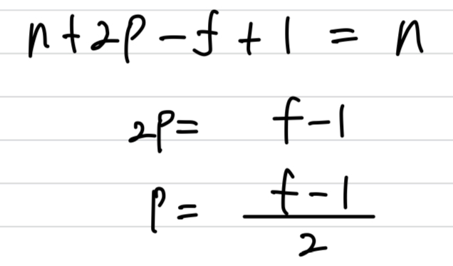
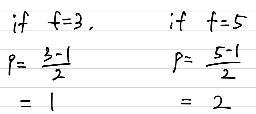
• And by convention in computer vision, $f$ is actually almost always odd(홀수).
  and you rarely see even numbered filters using computer vision.
  I think that two reasons for that.
  1. If $f$ is even, then you need some asymmetric padding. ($p = \frac{f-1}{2}$)
     If $f$ is odd, this type of same convolution gives a natural padding region,
     had the same dimension all around rather than pad more the left and pad less on the right,
     or something that asymmetric.
  2. When you have an odd dimension filter such as $3 * 3$ or $5 * 5$,
     then it has a central position and sometimes in computer vision its nice to have a distinguisher,
     it's nice to have a pixel you can call the central pixel so you can talk about the position of the filter.
     (홀수 크기의 필터의 경우 이전의 모든 층 픽셀은 출력 픽셀을 중심으로 대칭입니다.
     이러한 대칭이 없으면 짝수 크기의 커널을 사용할 때 나타나는 레이어 간의 왜곡을 설명해야 합니다.
     따라서 구현의 단순성을 높이기 위해 짝수 크기의 커널 필터는 대부분 생략됩니다.)

---

Strided Convolutions

• Strided Convolutions is another piece of the basic building block of convolutions as using convolutional neural networks.

• Let me show you an example.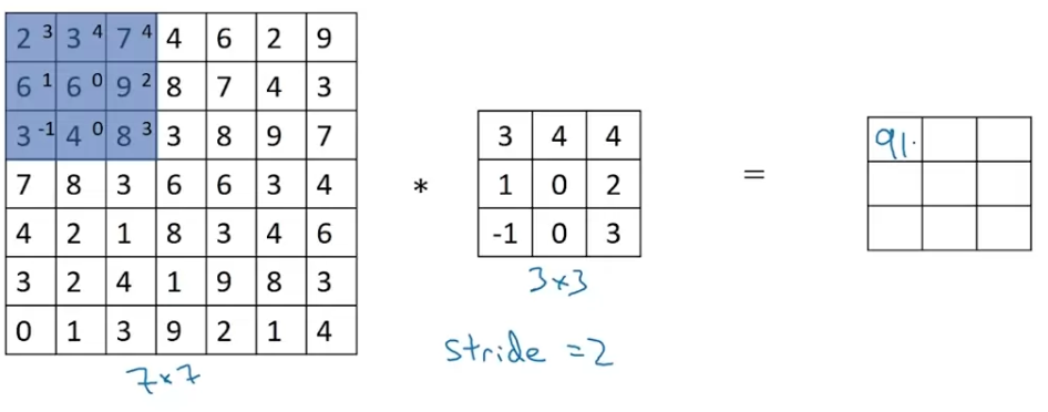we're going to step it over by two steps.
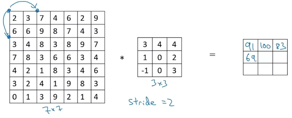
  If you have an $n$ x $n$ image convolve $f$x$f$ filter.
  If you use padding $p$ and stride $s$.
  In this example, $s=2$
  Then you end up with an output that is $(\frac{n + 2p -f}{s}+1)$ x $(\frac{n + 2p -f}{s}+1)$
  
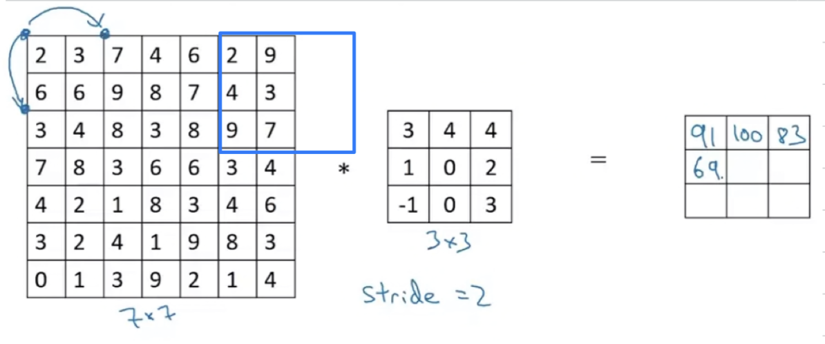
  Now one last detail which is one of this fraction is not an integer.
  In that case, we're going to round this $(\frac{n + 2p -f}{s}+1)$ down.
  If any of this blue box, part of it hangs outside then you just do not do that computation.
  Then the right thing to do, to compute the output dimension is to round down,
  in case this $\frac{n+2p-f}{s}$ is not an integer.
  

Summary of convolutions

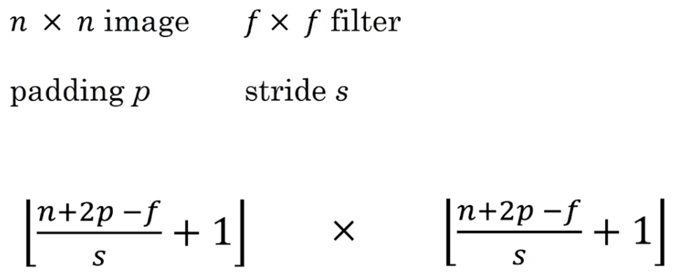
• Output size :

Technical note on cross-correlation vs convolution

• There is a technical comment i want to make about corss-correlation vs convolutions.
  This won't affect what you have to do to implement convolution neural networks.
  There is one other possible inconsistency in the notation.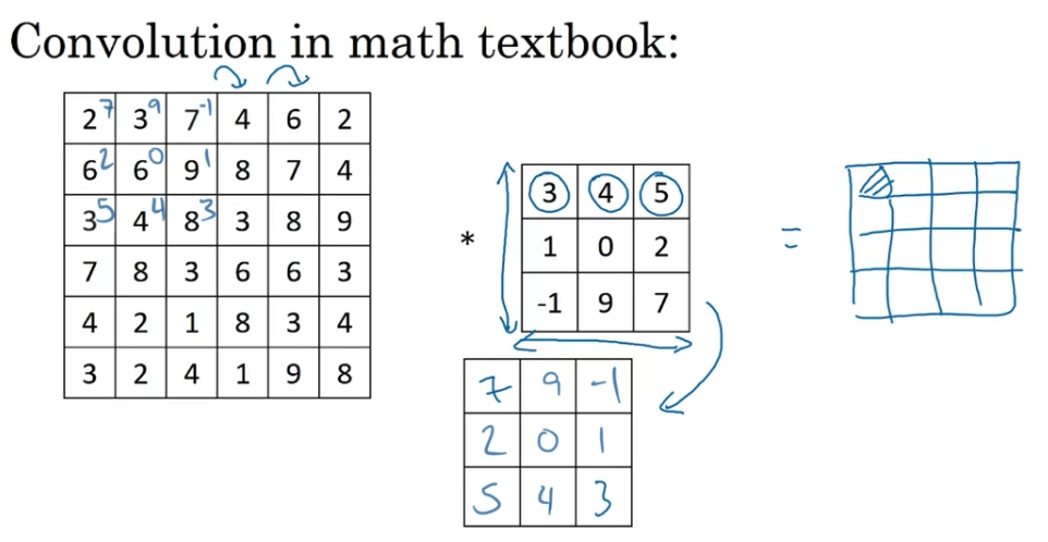
  before doing the element-wise product and summing,
  there's actually one other step that you would first take,
  which is to convolve this $6 * 6$ matrix and $3 * 3$ filter,
  and flip it on the horizontal as well as the vertical axis.
  
  To compute the output, you would take this flipped matrix.
  The way we've defined the convolution operation in these videos is that
  we've skipped this mirroring operation.
  And technically what we're actually doing?
  Really the operation we've been using for the last few videos
  is sometimes cross-correlation instead of convolution.
  That in the deep learning literature, by convention,
  we just call this the convolution operation
  
  So just to summarize,
  by convention, in machine learning, we usually do not bother with this flipping operation.
  And technically this operation is maybe better called cross-correlation.
  But most of the deep learning literature just causes the convolution operator.
  (원래 전통적인 신호처리에서 convolution은 신호를 뒤집은 후에 element-wise mul을 하고 sum하는 과정을 반복하고, cross-correlation은 신호를 뒤집지 않고 element-wise mul하고 sum하는 과정을 반복한다.
  CNN에서 convolution연산은 원래 cross-correlation인데, 관습적으로 그냥 convolution이라고 한다.)

---

Convolutions over volumes

• Now let's see how you can implement convolutions over not just 2D images
  but over 3 dimensional volumes.

Convolutions on RGB images

• Let's say you want to detect features, not just in a gray scale image.
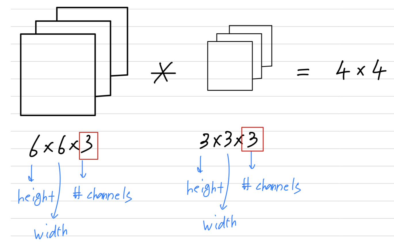  So RGB image might be $6$ x $6$ x $3$ where the $3$ responds to the three color channels.
  In order to detect edges or some other features in this image,
  you convolve this not with a $3 * 3$ filter as we have previously,
  now with also 3D filter that's going to be $3$ x $3$ x $3$.
  So the filter itself will also have $3$ layers corresponding to the red, green and blue channels.
  
  And the number of channels in your image must match the number of channels in your filter.
  We'll see on the next slide how this convolution operation actually works.

Convolutions on RGB image

• So here's the $6 * 6$ image,
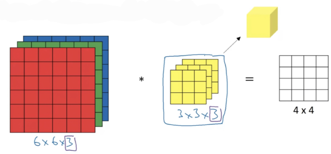  So to simplify the drawing of this $3 * 3 * 3$ filter,
  instead of drawing it as a stack of the matrices, just drawing it as this three dimensional cube.
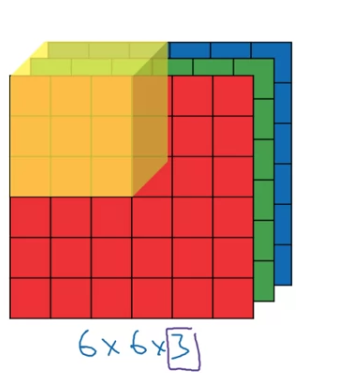
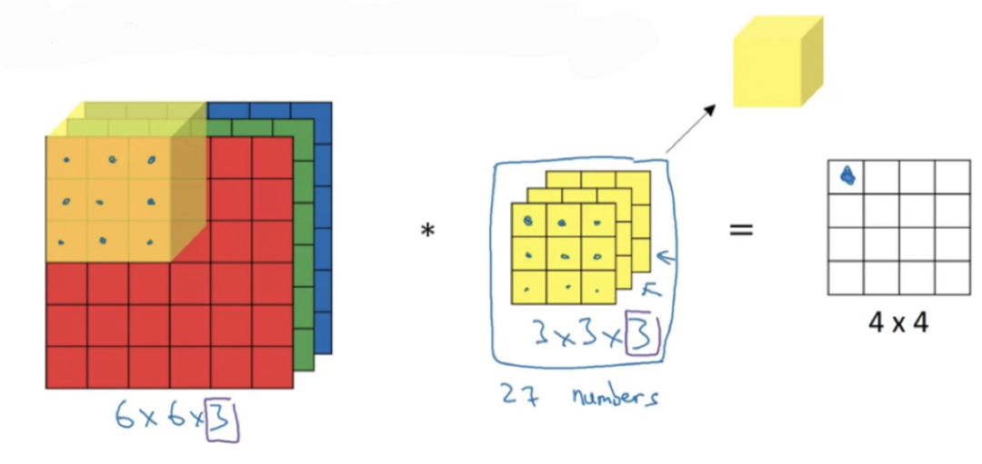  So to compute the output of this convolutional operation,
  what you would do is take the $3 * 3 * 3$ filter and first place it in that upper left most position.
  So notice that this $3 * 3 * 3$ filter = three cubes has $27$ parameters.
  And so what you do is take each of these $27$ numbers and multiply them with the corresponding numbers from the red, green, and blue channels of the image,
  then add up all those numbers and this gives you this first number in the output.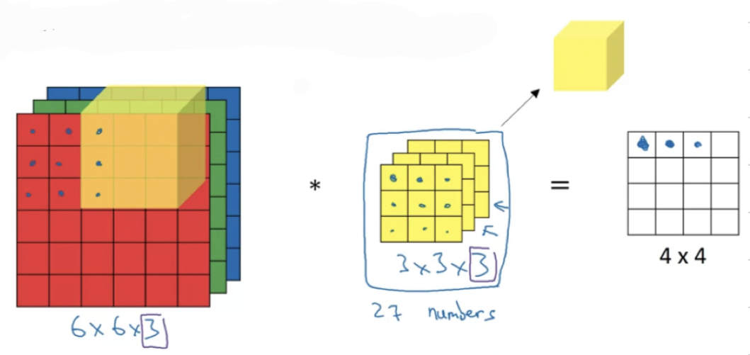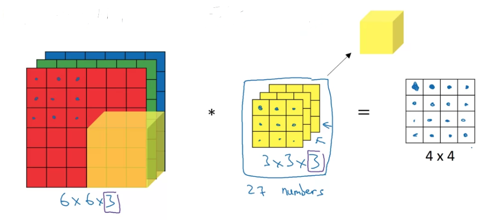and then to compute the next output you take this cube and slide it over by one,
  and again, due to $27$ multiplications, add up the $27$ numbers,
  that gives you next output.

• So what does this allow you to do?
  Here's an example.
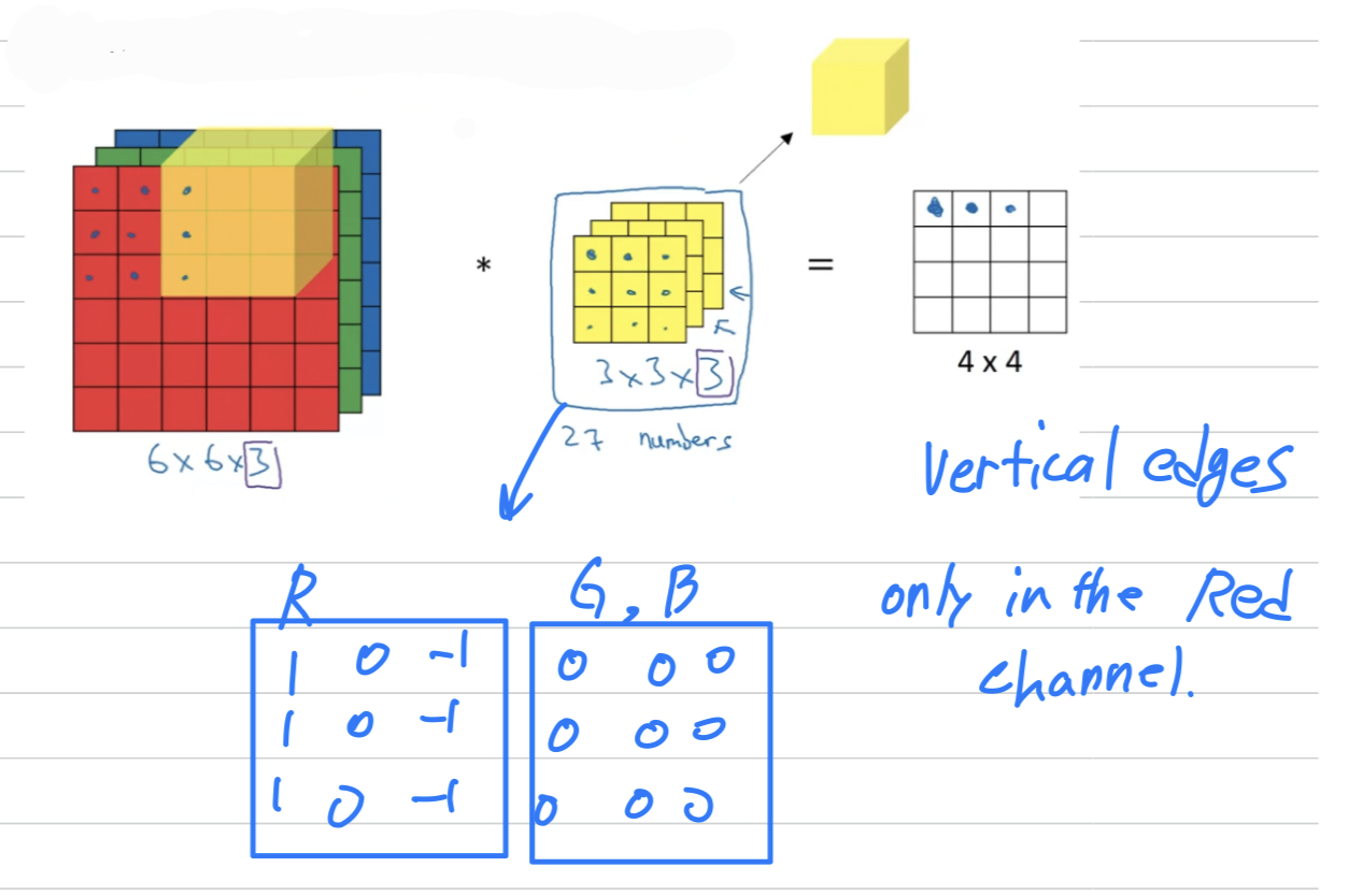  If you want to detect edges in the red channel of the image
  and have the green channel be all zeros
  and have the blue channel be all zeros.
  And if you have these stock together to form your $3 * 3 * 3$ filter,
  then this would be a filter that vertical edges but only in the red channel.
  
  And with different choices of these parameters
  you can get different features detectors out of this $3 * 3 * 3$ filter.
  
  And by convention, in computer vision,
  when you have an input with a certain height, a certain width, and a certain number of channels,
  then your filter will have a potentiall different height, different width, but the same number of channels.
  
  And once again, you notice that convolving a volume,
  a $6 * 6 * 3$ convolve with a $3 * 3 * 3$, that gives a $4 * 4$, a 2D output.

Multiple filters

• There's one last idea that will be crucial for building convolutional neural networks,
  which is what if we don't just wanted to detect vertical edges,
  what if we want to detect vertical edges and horizontal edges and maybe 34 degree edges and 70 degree edges as well,
  but in other words, what if you want to use multiple filters at the same time?
  (세로 edge만 detect하는 것이 아니라 세로와 가로 edge 모두를 detect하거나 기울기를 갖는 edge일 수도 있다,
  즉 여러 filter를 동시에 사용하려고 할 때는 어떻게 해야 하는가?)
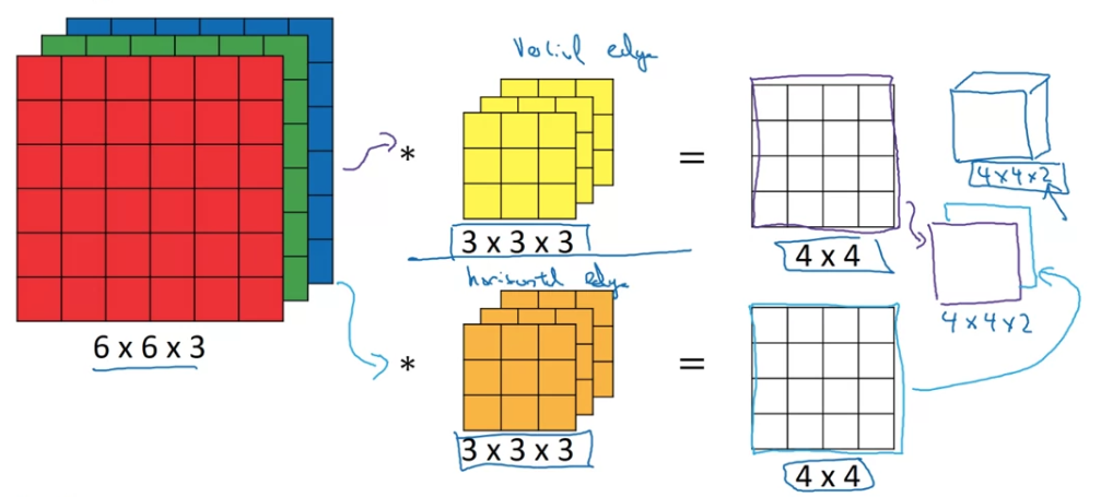  Let's say maybe this is a vertical edge detector,
  maybe a second filter is a horizontal edge detector.
  So maybe convolving it with the first filter gives you $4 * 4$ output
  and convolving with the second filter gives you a different $4 * 4$ output.
  
  And what we can do is then take these two $4 * 4$ outputs,
  take this first one within the front, and take this second filter output put it at back.
  so that by stacking these two together, you end up with a $4 * 4 * 2$ output volume.
  And the two here comes from the fact that we used two different filters.
  
  Even more important is that you can now detect two features, like vertical, horizontal edges,
  or 10 or maybe a 128 or maybe several hundreds of different features.
  And the output will have the number of channels(= the number of filters you are detecting).
  So, let's just summarize the dimensions,
  if you have $(n * n * n_C)$ input image where $n_C$ is the number of channels,
  and you convolve that with a $f * f * n_C$ where $n_C$ is the same number of input image's.
  Then, what you get is $(n-f+1) * (n-f+1) * n_C'$
  ($n'_C$ is the number of filters that you use == $n_C$ of next layer)

---

One Layer of a Convolutional Network

Example of one layer

• Get now ready to see how to build one layer of a convolutional neural network.
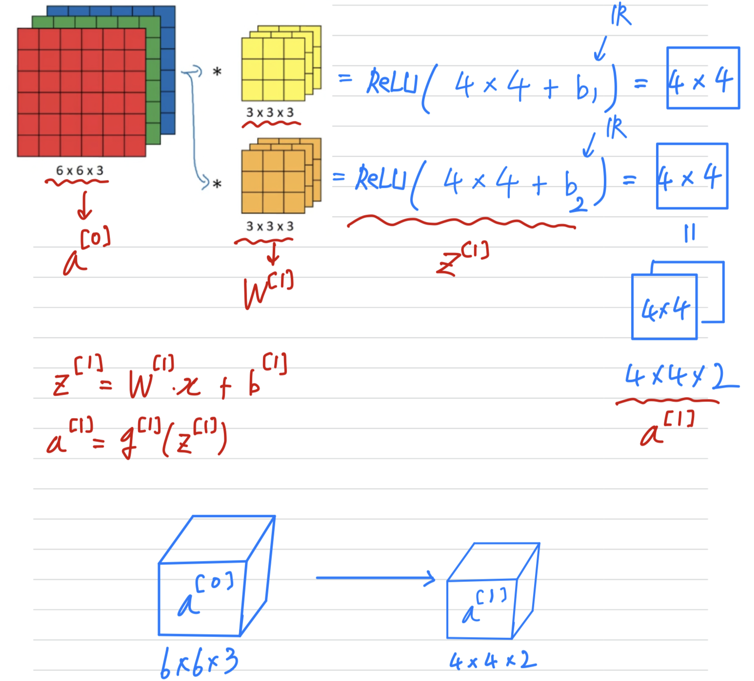  The final thing to turn this into a convolutional neural net layor
  is that for each of these we're going to add it bias,
  so bias is going to be a real number.
  
  Now in this example we have two filters,
  so we had two features which is why we end up with our output $4 * 4 * 2$.
  But if for example we instead had $10$ filters instead of $2$,
  then we would end up with the $4 * 4 * 10$ dimensional output volume.

Number of parameters in one layer.

• If you have $10$ filters that are $3 * 3 * 3$ in one layer of a neural network,
  how many prameters does taht layer here?
  • Each filter is a $3 * 3 * 3$ volume, so each filter has $27$ parameters.
    and plus the bias.
    So this gives you $28$ parameters.
    Then all together you'll have $28$ x $10 = 280$.
    
    Notice one nice thing about this,
    is that no matter how big the input image is but the number of parameters you have still remains fixed as $280$.
    And you can these $10$ filters to detect features, vertical edges, horizontal edges maybe other features even in a very large image
    is just a very small number of parameters.
    This is really one property of convolution neural network that makes less prone to overfitting if you could.
    (input image가 매우 커도 parameter의 수는 고정되기 때문에 적은 수의 변수로 feature detection이 가능하다.
    이것이 overfitting을 방지하는 Convolution neural network의 한 성질이다.)

Summary of notation

• If layer $l$ is a convolution layer :
  • $f^{[l]}$ = filter size
  • $p^{[l]}$ = padding
  • $s^{[l]}$ = stride
  • $Input$ : $n^{[l-1]}_H$ x $n^{[l-1]}_W$ x $n_C^{[l-1]}$
    • $n_H^{[l-1]} :$ height
    • $n_W^{[l-1]} :$ width
    • $n_C^{[l-1]} :$ the number of input channels
  • $Output$ : $n^{[l]}_H$ x $n^{[l]}_W$ x $n_C^{[l]}$
    • $n^{[l]}_H = floor(\frac{n^{[l-1]}_H + 2p^{[l]} -f^{[l]}}{s^{[l]}} + 1)$
    • $n^{[l]}_W = floor(\frac{n^{[l-1]}_W + 2p^{[l]} -f^{[l]}}{s^{[l]}} + 1)$
    • $n^{[l]}_C =$ the number of filters in layer $l$
  • $Activation$, $a^{[l]}$ : $n^{[l]}_H$ x $n^{[l]}_W$ x $n_C^{[l]}$
  • $Vectorized$ $Activation$, $A^{[l]}$ : $m * n^{[l]}_H$ x $n^{[l]}_W$ x $n_C^{[l]}$
  • $Each$ $filter$ : $f^{[l]} * f^{[l]} * n^{[l-1]}$
  • $Weights$ : $f^{[l]} * f^{[l]} * n^{[l-1]} * n^{[l]}_C$
  • $bias$ : $n^{[l]}_C$

---

Simple Convolutional Network Example

• Now let's go through a concrete example of a deep convolutional neural network.

Example ConvNet

• This would be a pretty typical example of a ConvNet.
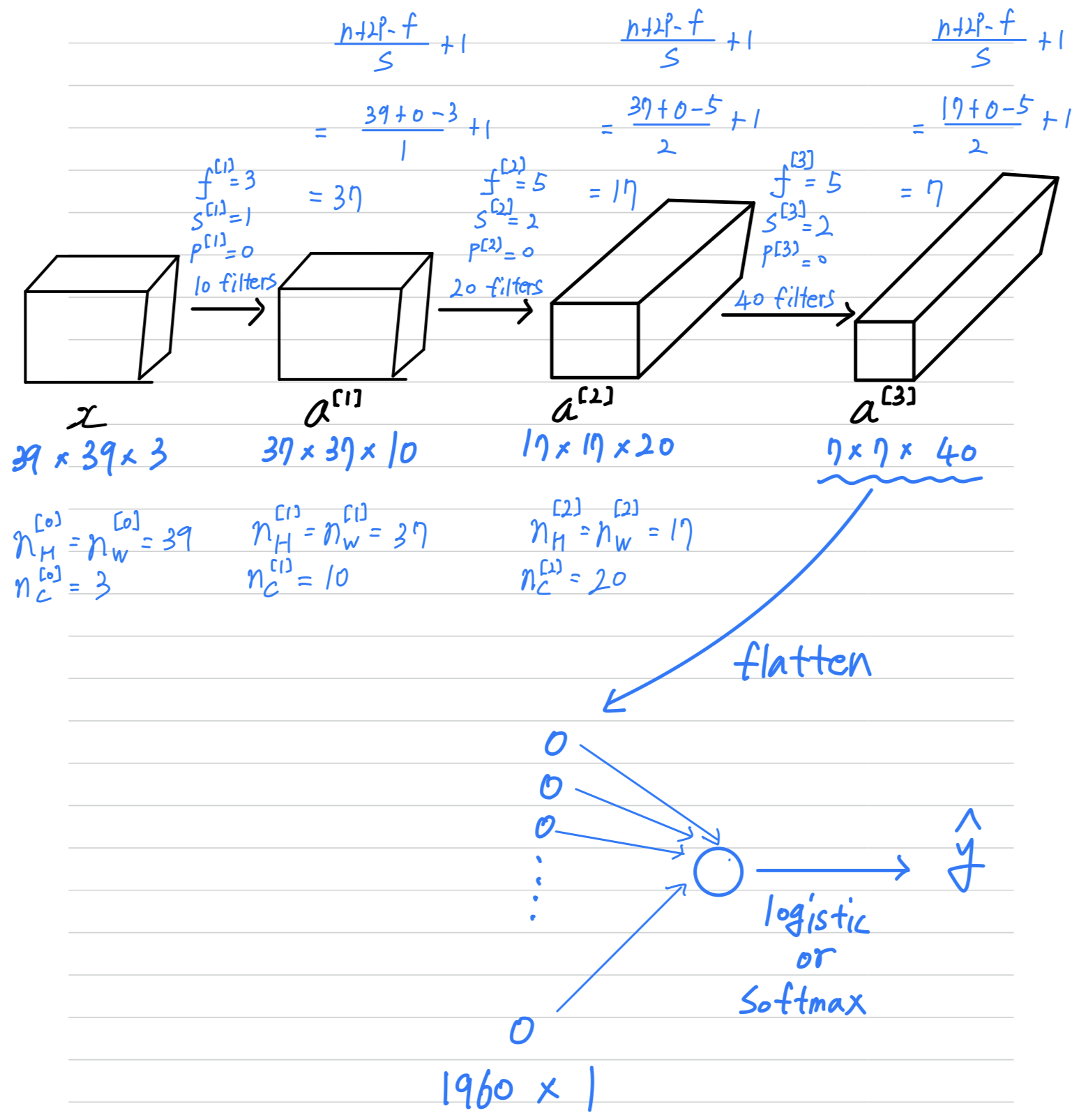  A lot of the work is designing convolutional neural net is selecting hyperparameters like these,
  deciding what's the total size? what's the stride? padding? and how many filters are used?
  And both later this week as well as next week,
  we'll give some suggestions and some guidelines on how to make these choices.
  
  But for now, maybe one thing to take away from this is that as you go deeper in a neural network,
  typically you start off with larger images, $39 * 39$.
  And then the height and width will stay the same for a while and gradually trend down as you go deeper in the neural network.
  It's gone from $39$ to $37$ to $17$ to $7$.
  Whereas the number of channels will generally increase.
  It's gone from $3$ to $10$ to $20$ to $40$.
  and you see the general trend in a lot of other convolutional neural networks as well.
  

Types of layer in a convolutional network

• It turns out that in a typical ConvNet,
  there are usually three types of layers.
  1. Convolutional layer = Conv : That's what we've been using in the previous network.
  2. Pooling layer = Pool : we'll talk about in the next videos.
  3. Fully connected layer = FC : we'll talk about in the next videos.
• Pooling layer and Fully connected layer are a bit simpler than convolutional layers to define.
  So we'll do that quickly in the next two videos
  and then you have a sense of all of the most common types of layaers in a convolutional neural network.
  And you will put together even more powerful networks than the one we just saw.

---

Pooling layers

• Other than convolutional layers,
  ConvNets often also use pooling layers to reduce the size of the representation to speed up the computation,
  as well as make some of the features that detects a bit more robust.
  

Pooling layer : Max pooling

• Let's go through an example of pooling, and then we'll talk about why you might want to do this.
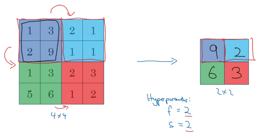
  So to compute each of the numbers on the right,we took the max over a $2 * 2$ regions.
  So this is as if you apply $f = 2$ because you're taking a $2 * 2$ regions
  and you're taking a $s = 2$
  So these are actually the hyperparameters of max pooling.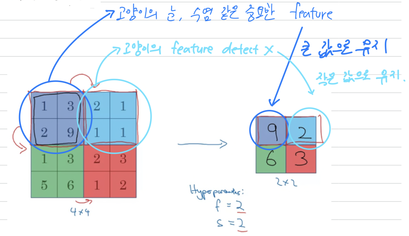So here's the intuition behind what max pooling is doing.
  If you think of this $4 * 4$ region as some set of features,
  the activations in some layer of the neural network,
  then a large number, it means that it's maybe detected a particular feature.
  So the upper left-hand quadrant has this particular feature,
  it maybe a vertical edge or maybe a higher or whisker if you detect a cat.
  Clearly, that feature exists in the upper left-hand quadrant.
  Whereas this feature, it doesn't really exist in the upper right-hand quadrant.
  
  So what the max operation does is a lots of features detected anywhere,
  and one of these quadrants, it then remains preserved in the output of max pooling.
  So what the max operates to does is really to say,
  if these features detected anywhere in this filter, then keep a high number.
  But if this features is not detected, so maybe this feature doesn't exist in the upper right-hand quadrant,
  then the max of all those numbers is still itself quite small.
  So maybe that's the intuition behind max pooling.
  
  I don't know of anyone fully knows if that is the real underlying reason that max pooling works well in ConvNets.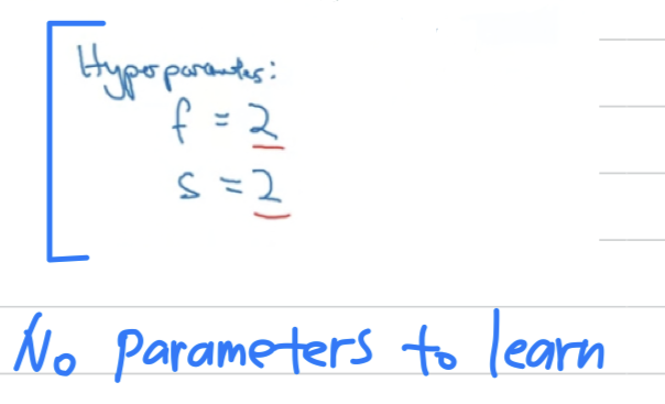One interesting property of max pooling is that it has a set of hyperparameters
  but it has no parameters to learn.
  Once you fix $f$ and $s$, it's just a fixed computation and gradient descent doesn't change anything.

• Let's go through an example with some different hyperparameters.
  Max pooling on a 2D inputs :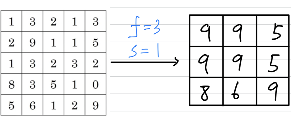 If you have 3D input, then the output will have the same dimension : 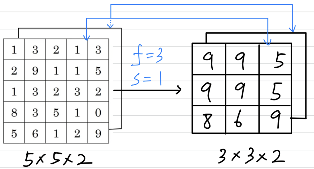The way you compute max pooling is you perform the computation
  we just described on each of the chaneels independently.
  And more generally, if this $5 * 5 * n_C$ the output would be $3 * 3 * n_C$.
  The max pooling computation is done independently on each of these $n_C$ channels.

Pooling layer : Average pooling

• Average pooling is one of the types of pooling that isn't used very often.
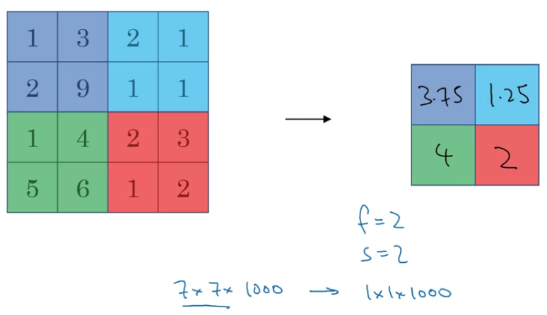  You see max pooling used much more in the neural network than average pooling.

Summary of pooling

• So just to summarize,
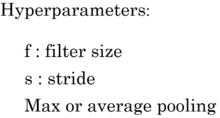  Maybe common choices of parameters might be $f=2$, $s=2$.
  This is used quite often and this has the effect of roughly shrinking the height and width by a factor of above two.
  (높이와 너비를 절반정도로 축소시키는 효과.)
  
  I've also seen $f=3$, $s=2$ used,
  and then the other parameter is just like a binary bit,
  that says are you using max pooling? or are you using average pooling?
  
  If you want, you can add an extra hyperparameter for the padding although this is very, very rarely used.
  When you do max pooling, usually you do nt use any padding
  although there is one exception that we'll see next weel as well.
  So the most common value of $p=0$.
  
  Assuming there's no padding
  and the input of max pooling is that you input a volume of size that $n_H * n_W * n_C$,
  and it would output a volume of size given by $floor(\frac{n_H - f}{s}+1) * floor(\frac{n_W - f}{s}+1) * n_C$
  
  One thing to note about pooling is that there are no parameters to learn.
  So when we implement back prop, you find that there are no parameters that backprop will adapt through max pooling.

---

CNN Example

Neural network example

• You're trying to do handwritten digit recognition.
  Let's throw the neural network to do this.

  It's actually quite similar to one of the classic neural networks called LeNet-5,
  which is created by Yann LeCun many years ago.
  What i'll show here isn't exactly LeNet-5, but many parameter choices were inspired by it.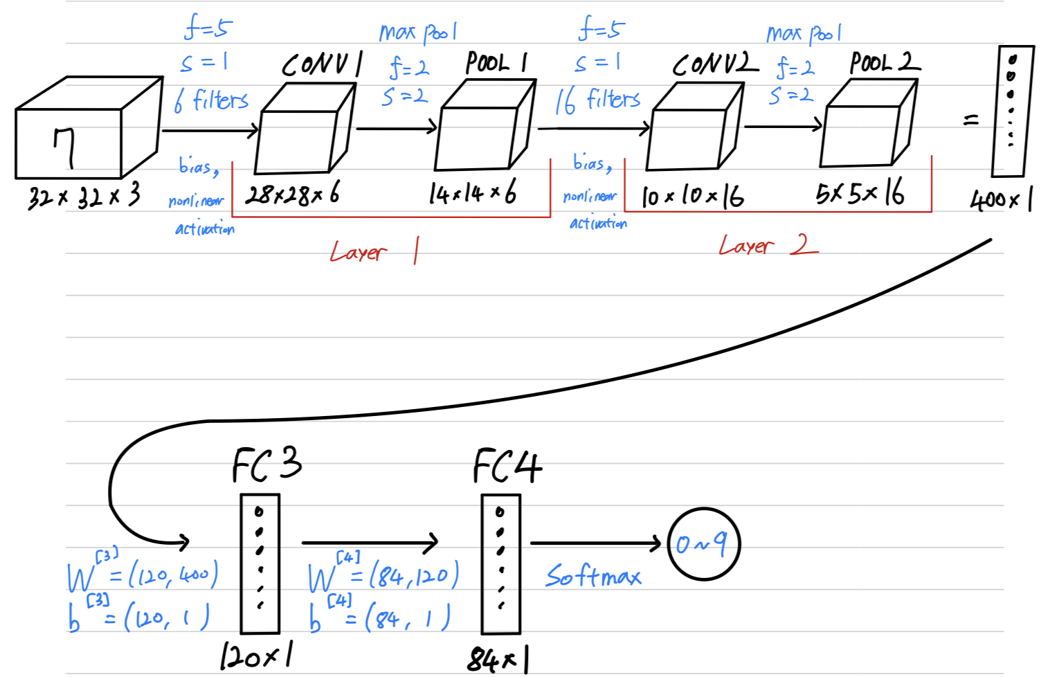
  When people report the number of layers in a neural network,
  people report the number of layers that have weight, that have parameters.
  And because the pooling layer has no weights, has no parameters, only a few hyper parameters,
  I'm going to use a convention that CONV1 and POOL1 shared together.
  I'm going to treat that as Layer 1
  although sometimes you see people if you read articles online and read research papers,
  you hear about the conv layer and the pooling layer as if they are two separate layers.
  But when i count layers, i'm just going to count layers that have weights.
  So we treat both of CONV layer and POOL both as Layer 1.
  
  Pointed this out earlier, but it goes from $32 * 32$ to $28 * 28$ to $14 * 14$ to $10 * 10$ to $5 * 5$.
  So as you go deeper usually the height and width will decrease,
  whereas the number of channels will increase.
  It's gone from $3$ to $6$ to $16$ and then your fully connected layer is at the end.
  
  And another pretty common pattern you see in neural networks is
  to have one or more conv layers followed by a pooing layer,
  and then one or more conv layers followed by pooling layer,
  ...
  and then at the end you have a fully connected layers
  and then followed by maybe a softmax.
  (CONV - POOL - ... - CONV - POOL - FC - ... - FC - Softmax)

  • So let's just go through for this neural network some more details of
    what are the activation shape, the activation size, and the number of parameters in this network.

    First, notice that the max pooling layers don't have any parameters.
    Second, notice that the conv layers tend to have relatively few parameters,
    and a lot of parameters tend to be in the fully connected layers of the neural network.
    And then you notice also that the activation function size tends to go down gradually as you go deeper in the neural network.
    If activation size drops too quickly, that's usually not great for performance as well.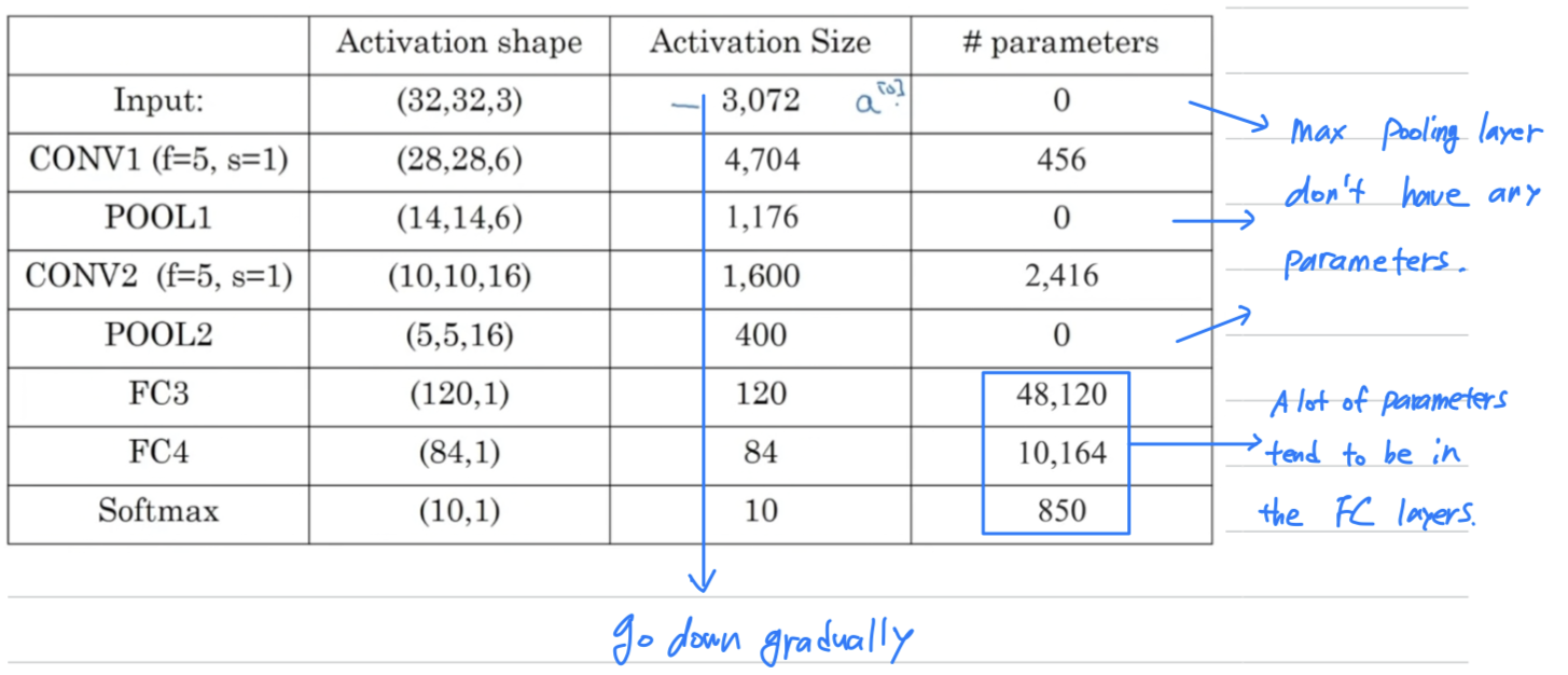A lot of computer vision research has gone into figuring out how to put together
    these basic building blocks to build effective neural networks.
    I think one of the best way for you to gain intuition is about how to these things together is
    a see a number of concrete examples of how others have done it.

---

Why Convolutions?

• Let's talk about why convolutions are so useful when you include them in your neural networks.
  And then finally, let's talk about how to put this all together and how you can train a convolutional neural network when you have a label training set.
  
• I think there are two main advantages of convolutional layers over just using fully connected layers.
  And the advantages are parameter sharing and sparsity of connections.
  Let me illustrate with an example.
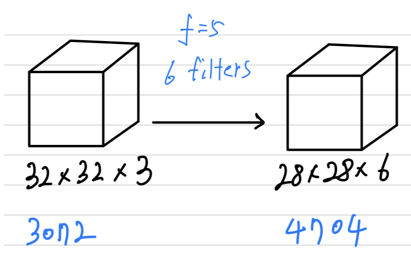
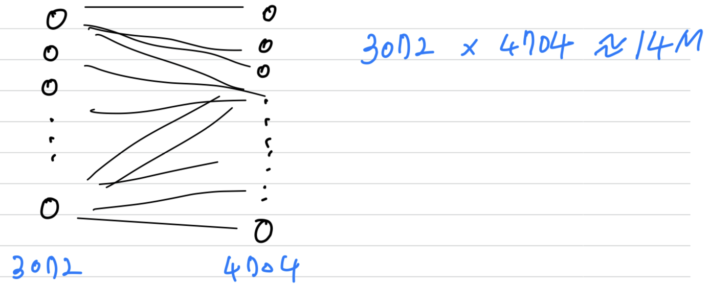  And so, if you were to create a neural network with $3,072$ units in one layer, and with $4,704$ units in the next layers and if you were connect every one of these neurons,
  then the the number of parameters in a weight matrix would be $3,072$ x $4,704$ which is about $14$ $millions$.
  So that's just a lot of parameters to train.
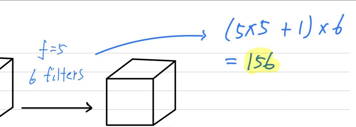  But if you look at the number of parameters in this convolutional layer,
  each filter is $5 * 5$.
  So each filter has $25$ parameters + a bias parameters = $26$ parameters per a filter,
  and you have $6$ filters, so the total number of parameters is that which is equal to $156$ parameters.
  And so the number of parameters in this conv layer remains quite small.
  
  And the reason that a conv net has run to these small parameters is really two reasons.

1. Parameter sharing : Parameter sharing is motivated by the observation that feature detector such as vertical edge detector that's useful in one part of the image is probably useful in another part of the image.
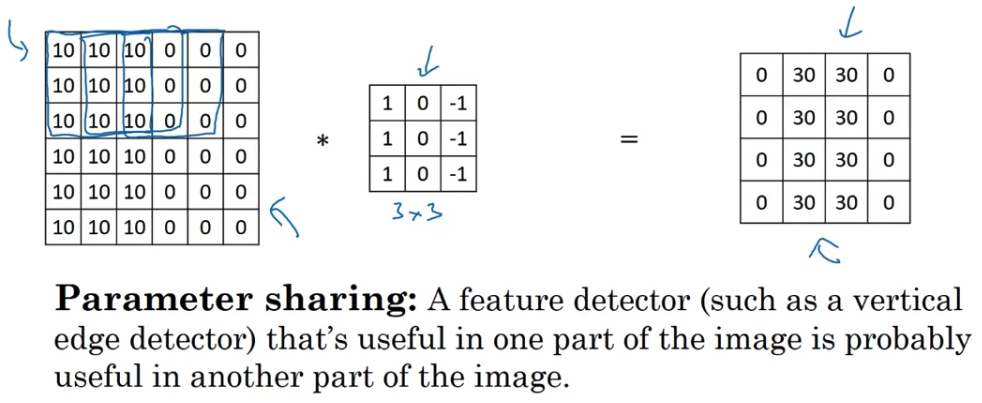   If you've figured out say a $3 * 3$ filter for detecting vertical edges,
   you can then apply the same $3 * 3$ filter over here
   and then the next position over here,
   and the next position over, and so on.
   Each of these feature detectors, each of these outputs can use the same parameters in lots of different positions in your input image
   in order to detect say a vertical edge or some other feature.
   
   And i think this is true for low-level features like edges,
   as well as the higher level features like maybe detecting the eye that indicates a face or a cat or something there.
   
   But being with a share in this case
   the same $9$ parameters to compute all $16$ of these outputs,
   is one of the ways the number of parameters is reduced.
   
   And it also just seems intuitive that a feature detector like a vertical edge detector
   computes it for the upper left-hand corner of the image.
   The same feature seems like it will probably has a good chance of being useful for the lower-right hand corner of the image.
   So you don't need to learn separate feature detectors for the upper left and the lower right-hand corners of the image.
   
   And maybe you do have a dataset where you have the upper-right hand corner and lower right-hand corner have different distributions.
   So they maybe look a little bit different but they might be similar enough,
   they're sharing feature detectors all across the image, works just fine.
   ($3 * 3$ filter 즉, feature detector로 input image에서 해당하는 feature를 detection하도록 하여
   똑같은 parameter를 사용하여 feature를 detection할 수 있다.
   따라서 이를 통해 parameter 수를 줄일 수 있다.)

2. Sparsity of connections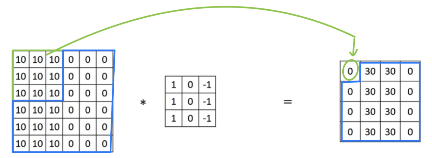 : If you look at this zero, this is comptued via $3 * 3$ convolution.
   And so it depends only on this $3 * 3$ inputs gride or cells.
   So as if this output unit(=0) is connected only to $3 * 3$ of $9 * 9$ input features
   And in particular, the rest of these pixel values do not have any effects on the other output.
   
   Through this mechanism,
   a neural network has a lot fewer parameters which allows it to be trained with smaller training cells and is less prone to be overfitting.
   
   And so sometimes you also hear about
   convolutional neural network being very good at capturing translation invariance.
   And that's observation that a picture of a cat shifted a couple of pixels to the right is still pretty clearly a cat.
   And convolutional structure helps the neural network encode the fact that an image shifted a few pixels
   should result in pretty similar features and should probably be assigned the same output label.
   And the fact that you are applying to same filter, all the positions of the image,
   both in the early layers and in the late layers that helps a neural network automatically learn to be more robust or to better capture the desirable property of translation invariance.
   (동일한 크기의 filter를 input image의 모든 position에 적용하기 때문에 image에서 고양이가 오른쪽으로 이동했어도 자동으로 feature를 detection할 수 있다.
   이를 변환 불변성 = translation invariance.)
   
   

Putting it together

• Finally, let's put it all together and see how you can train one of these networks.
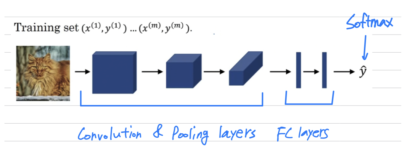
  where now $x$ is an image and the $y$ can be binary labels or one of $K$ classes.
  The conv layers and the fully connected layers will have various parameters $W$ as well as bias $b$.
  And so any setting of the parameters, therefore, let's you define a cost function
  where we've randomly initialized parameters $W, b$.
  You can compute the cost $J$
  as the sum of losses of the neural networks predictions on you entire training set, maybe divide it by $m$.
  So to train this neural network,
  all you need to do is then use gradient descent or some of the algorithm like gradient descent momentum, or RMSProp or Adam, or something else
  in order to optimize all the parameters of the neural network to try to reduce the cost function $J$.
  And you find that if you do this,
  you can build a very effective cat detector or some other detector.

---

Seminar - discussion

• logit은 마지막 layer의 $z$값임.
  logit은 $Z_3$이며, 확률이 아님.
  from_logits=True ➡️ 확률로 normalize가 아직 되지 않은 것 == 확률로 되지 않은 것들의 Cross Entropy를 계산해줘라.
  from_logits=False ➡️ 0~1 확률로 normalize된 것들 == logits이 아닌 것들의 Cross Entropy를 계산해줘라.

• 언어, 말과 관련된 모델을 Sparsity of connection이 효과가 있다.
  언어 데이터는 모든 data가 필수적이기 때문이다.
  따라서 언어 model에 CNN을 쓸 수는 있지만 보통 언어 전체를 볼 수 있는 필터인 Transformer를 사용한다.
  Transformer은 text 앞에 있는 단어와 맨 끝에 있는 단어까지 모두의 상관관계를 따진다.
  따라서 Sparsity of connection의 특징을 잘 살린 영상처리에 효과적이다.
  ➡️ 입력되는 data의 특성에 따라 model의 구성이 완전히 달라진다.
  영상처리에 특화된 model을 만들기 위해 CNN이 개발된 것이다.