Why look at case studies?

• Why look at case studies?
  It turns out the past few years of computer vision research has been on how to put together these basic building blocks(convolutional layers, pooling layers, fully connected layer) to form effective convolutional neural networks.
  
  One of the best ways for user gain intuition yourself is to see some of these examples.

• Outline

  • Classic networks :
    • LeNet-5
    • AlexNet
    • VGG
  • ResNet(=Residual Network) : The ResNet trained a very deep 152 layer neural network.
  • Inception

After seeing these neural networks,
i think you have much better intuition about how to build effective convolutional neural networks.

Classic networks

LeNet-5

• The goal of LeNet-5 was to recognize handwritten digits.
  And LeNet-5 was trained on grayscale images.
  
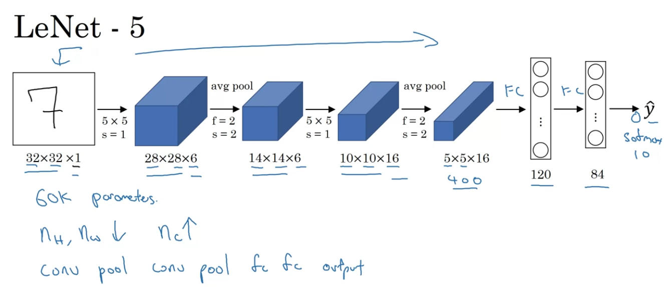
  • Back then when this paper was written, people use average poolig much more.
    If you're building a modern variant, you probably use max pooling instead.
  • And back when this paper was written in 1998,
    people didn't really use padding or you always using valid convolutions.
  • $\hat{y}$ took on $10$ possible values corresponding to recognizing each of the digits from $0$ to $9$.
    A modern version of this neural network, we'll use a softmax layer with a $10$ way classification output.
    Although back then, LeNet-5 actually use a different classifier at the output layer, one that's useless today.
  • So this neural network was small by modern standards, had about $60,000$ parameters.
    And today, you often see neural networks with anywhere from $10 million$ to $100 million$ parameters, and it's not unusal to see networks that are literally about a thousand times bigger than this network.
  • One thing you do see is that as you go deeper in a network, so as you go from left to right,
    the height and width tend to go down(32 ➡️ 28 ➡️ 14 ➡️ 10 ➡️ 5)
    , whereas the number of channels does increase(1 ➡️ 6 ➡️ 16)
  • One other pattern you see in this neural network that's still often repeated today is that you might have some one or more CONV layers followed by POOLING layer, ..., and then some FC layers and then the outputs.
• Few more advanced comments
  
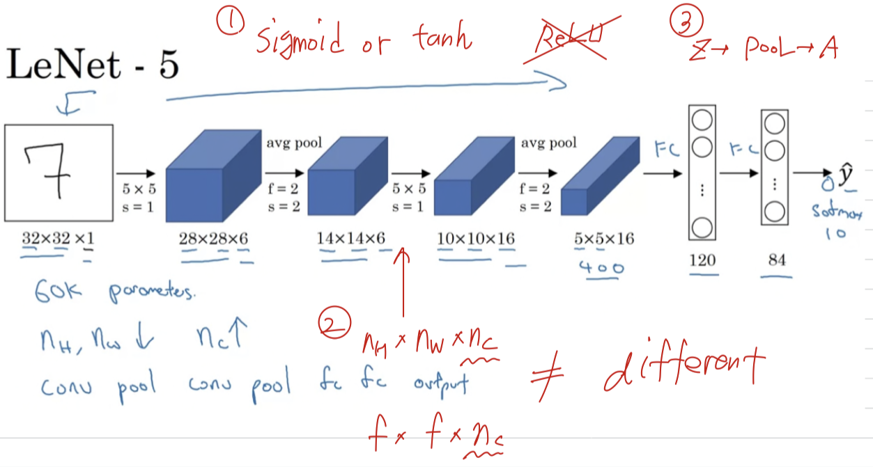
  • It turns out that if you read the original paper,
    people used sigmoid and tanh nonlinearities, and people weren't using ReLU nonlinearities back then.
    So if you look at the paper, you see sigmoid and tanh referred to.
  • 현대 표준으로 볼 때, 우스운 network이다.
    For example, activation으로 $(n_H * n_W * n_C)$ 가 있다고 할 때, filter도 $(f * f * n_C)$ dimension일 것이다.
    But back then, computers were much slower.
    And so save on computation as well as some parameters, the original LeNet-5 had some crazy complicated way where different filters would look at different channels of the input block.
    그래서 논문에서는 이러한 detail을 말하고 있다.
    하지만 modern implementation에서는 그러한 complexity는 없다.
  • The original LeNet-5 had a non-linearlity after pooling,
    and i think it actually uses sigmoid non-linearity after the pooling layer.

AlexNet

• AlexNet named after Alex Krizhevsky, who was the first author of the paper describing this work.
  The other author's were llya Sutskever and Geoffrey Hinton.

• AlexNet input starts with $227 * 227 * 3$ images.
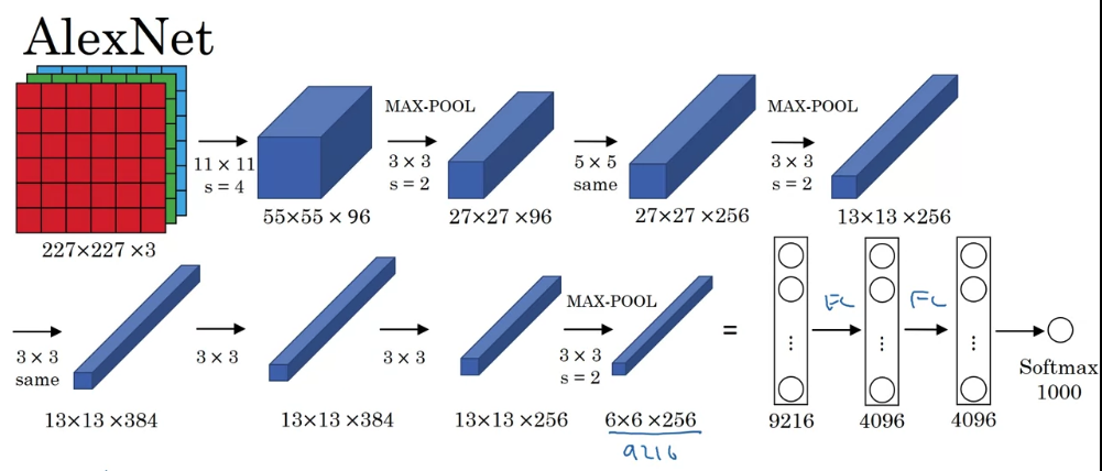  And if you read the paper, the paper refers to $224 * 224 * 3$ images.
  And then finally, it uses a softmax to output which one of $1000$ classes the object could be.

  • So this neural network actually had a lot of similarities to LeNet, but it was much bigger.
    The LeNet-5 had about $60,000$ parameters, this AlexNet had about $6,000,000$ parameters.
    And the fact that they could take pretty similar basic building blocks but have a lot more hidden units and training on a lot more data,
    they trained on the image that dataset that allowed it to have a remarkable performance.
  • Another aspect of this architecture that made it much better tan LeNet was using the ReLU activation function.

• Few more advanced comments

  • When this paper was written, GPUs was still a little bit slower,
    so it had a complicated way of training on two GPUs.
    And the basic idea was that, a lot of these layers was actually split across two different GPUs and there was a thoughful way when the two GPUs would communicate with each other.
    (두 개의 서로 다른 GPU로 분할되어 있으며, 두 GPU가 서로 통신할 수 있는 시기를 고려하여 신중하게 조정되었다.)
  • The original AlexNet architecture also had another type of a layer called a Local Response Normalization.
    And this type of layer isn't really used much.
    let's say for the sake of argument $13 * 13 * 256$,
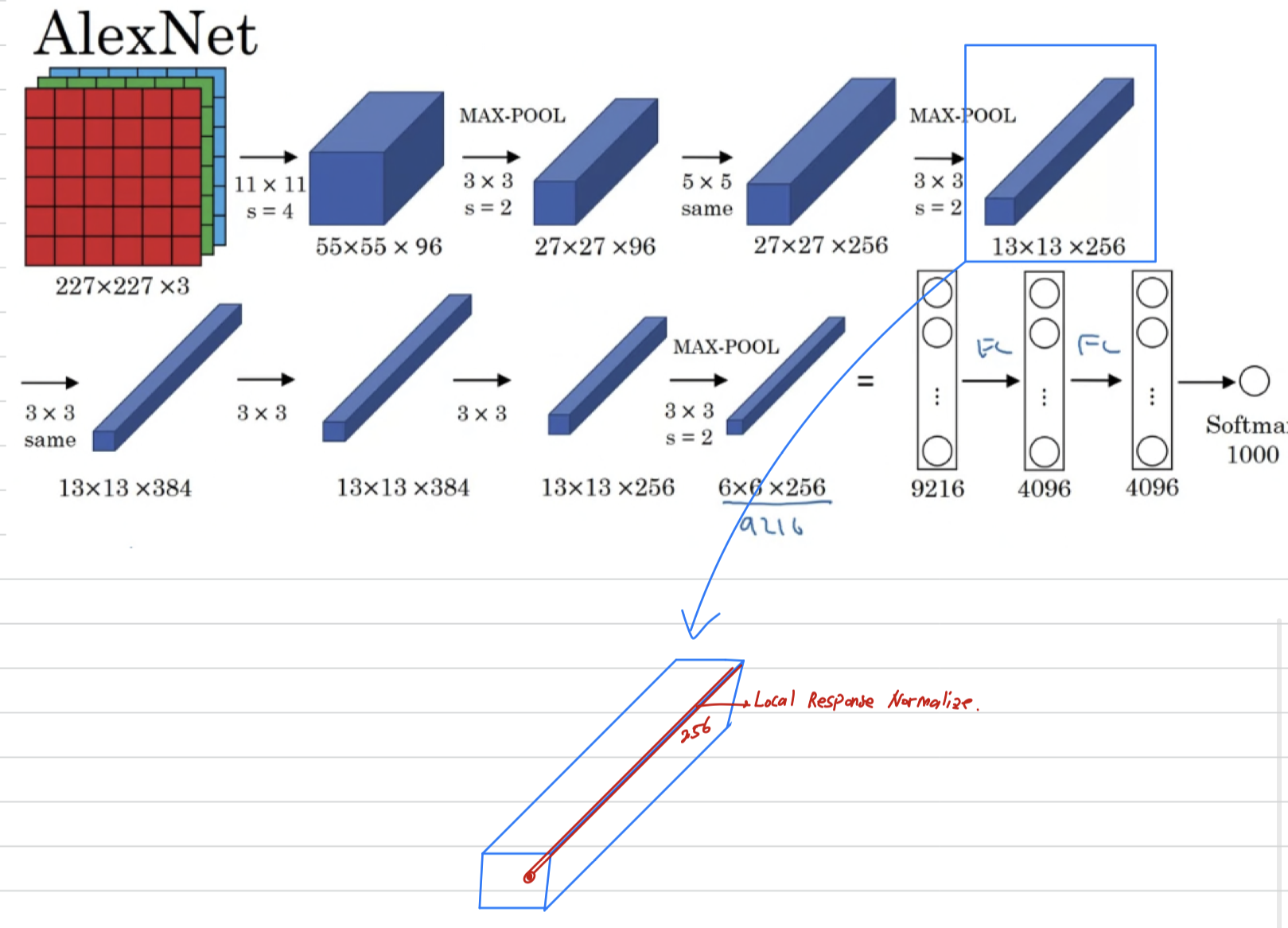    what Local Response Normalization does, is you look at one position.
    So one position height and width, and look down this across all the channels,
    look at all $256$ numbers and normalize them.
    And the motivation for this LRN was that for each position in this $13 * 13$ image,
    maybe you don't want too many neurons with a very high activation.
    But subsequently, many researchers have found that this doesn't help that much.

VGG-16

• VGG or VGG-16 net is that they said instead of having so many hyperparameters,
  let's use a much simpler network where you focus on just having conv-layers
  that are just $3 * 3$ filters with a $s=1$ and always use same padding.
  And make all your max pooling layers $2 * 2$ with a $s=2$.
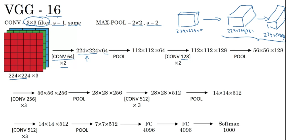  The $16$ in the VGG-16 refers to the fact that this has $16$ layers that have weights.
  This network has a total of about $1,380,000$ parameters.
  And that's pretty large even by modern standards. (현대 기준으로 봐도 꽤 큼)
  But the simplicity of the VGG-16 architecture made it quite appealing.
  I think the relative uniformity of this architecture made it quite attractive to researchers. (균일화된 것이 매력적임)
  But the main downside was that it was a pretty large network in terms of the number of parameters you had to train.
  
  And if you read the literature, you sometimes see people talk about the VGG-19, that is an even bigger version of this network.
  But because VGG-16 does almost as well as VGG-19, a lot of people will use VGG-16.

만약 위 Classic Networks에 대한 논문을 읽을 거라면,
AlexNet ➡️ VGG net ➡️ LeNet 순으로 읽는 것이 좋을 것이다.

---

ResNets

• Very, very deep neural networks are difficult to train, because of vanishing and exploding gradient types of problems.
  In this video, you'll learn about skip connections which allows you to take the activation from one layer and suddenly feed it to another layer even much deeper in the neural network.
  And using that, you'll build ResNet which enables you to train very, very deep networks.
  Sometimes even networks of over $100$ layers.

• ResNets are built out of something called a residual block,
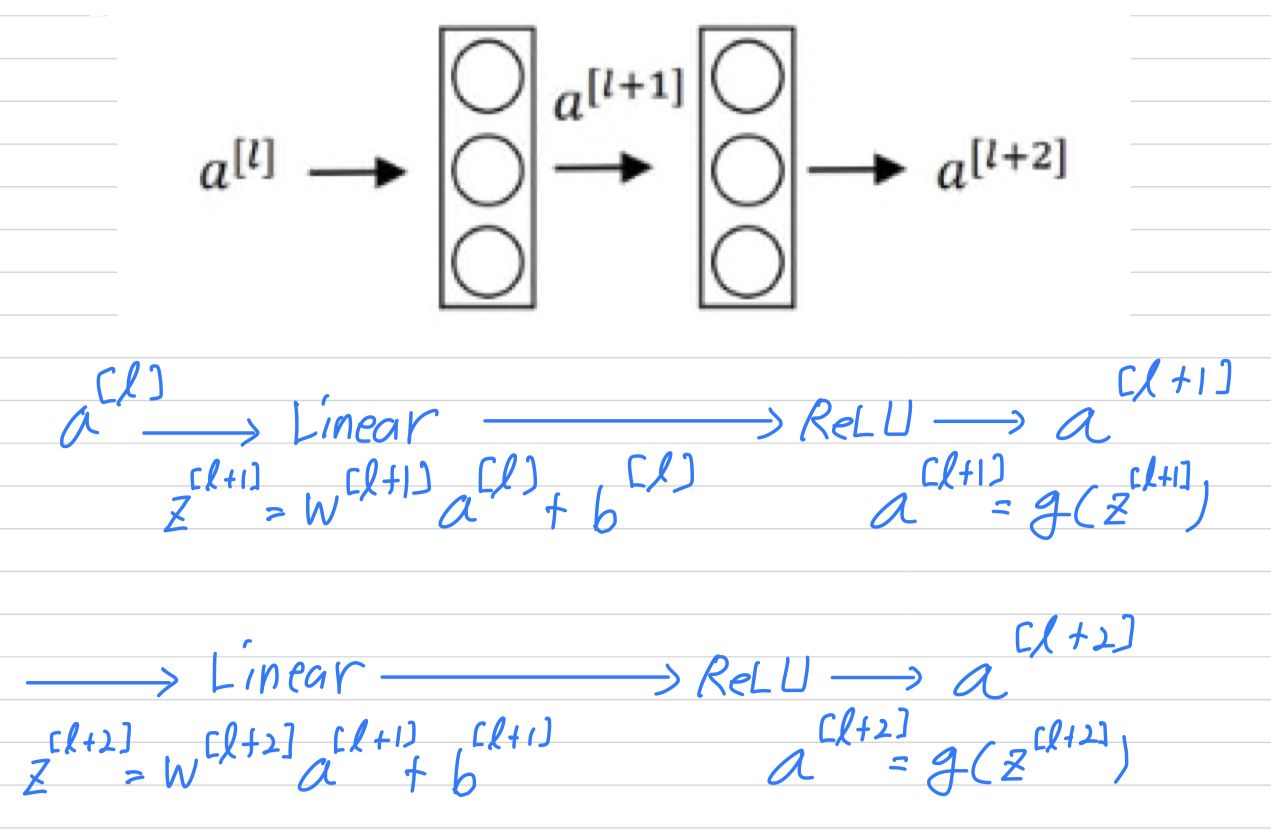  Here are two layers of a neural network where you start off with some activations in layer $a^{[l]}$,
  then goes $a^{[l+1]}$ and then the activation two layers later is 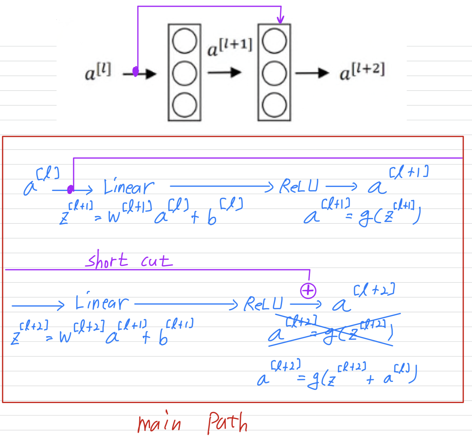$a^{[l+2]}$.So in other words, for information from $a^{[l]}$ to flow to $a^{[l+2]}$,
  it needs to go through all of these steps wthich i'm going to call the main path of this set of layers.
  In a residual net, we're going to make a change to this.
  We're going to take $a^{[l]}$, and just first forward it, copy it, match further into the neural network to $z^{[l+2]}$, and just add $a^{[l]}$ before applying to ReLU non-linearity.
  And i'm going to call this the shortcut.
  
  So rather than needing to follow the main main path,
  the information from $a^{[l]}$ can now follow a shortcut to go much deeper into the neural network.
  
  So, what the inventors of ResNet, that'll be Kaiming He, Xiangyu Zhang, Shaoqing Ren and Jian Sun.
  What they found was that using residual blocks allows you to train much deeper neural networks.

Residual Network

• And the way you build a ResNet is by taking many of these residual blocks,
  and stacking them together to form a deep network.
  So let's look at this network.
  This is not the residual network, this is called as a plain network.
  This is the terminology of the ResNet paper.
  To turn this into a ResNet, what you do is you add all those skip connections although those short like a connections like so.
  So every two layers ends up with that additional change that we saw on the previous slide to turn each of these into residual block.
  So this picture shows five residual blocks stacked together, and this is a residual network.
  
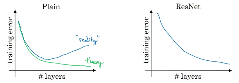  And it turns out that if you use your standard optimization algorithm such as a gradient descent or one of the fancy optimization algorithms to train the plain network.
  So without all the extra residual, without all the extra short cuts or skip connections.
  Empirically, you find that as you increase the number of layers,
  the training error will tend to decrease after a while but then they'll tend to back up.
  And in theory as you make a neural network deeper, it should only do better and better on the training set.
  
  But in practice or in reality, having a plain network, so no ResNet,
  having a plain network that is very deep means that all your optimization algorithm just has a much harder time training.
  And so, in reality, your training error gets worse if you pick a network that's too deep.
  But what happens with ResNet is that even as the number of layers gets deeper, you can have the performance of the training error kind of keep on going down.
  Even if we train a network with over a $100$ layers.
  But by taking these activations be it $X$ or those intermediate activations and allowing it to go much deeper in the neural network,
  this really helps with the vanishing and exploding gradient problems and allows you to train much deeper neural networks without really appreciable loss in performance,

Why do residual networks work?

• What we saw on the last video was that if you make a network deeper,
  it can hurt your ability to train the network to do well on the training set.
  And that's why sometimes you don't want a network that is too deep.
  But this is not true or at least is much less true when you training a ResNet.
  (network가 deep할수록 train이 잘 되지 않았는데 ResNet을 사용한다면 그렇지 않을 수 있다.)

• Let's say you have $X$ feeding in to some big neural network and just outputs some activations $a^{[l]}$
  Let's say for this example that you are going to modify the neural network to make it a little bit deeper.
  So, use the same big NN, and this output's $a^{[l]}$,
  and we're going to add a couple extra layers to this network.
  And this will output $a^{[l+2]}$.
  Only let's make this a residual block with that extra short cut.And for the sake our argument, let's say throughout this network we're using the ReLU activation functions.
  So all the activations $a >= 0$ with the possible exception of the input $X$.
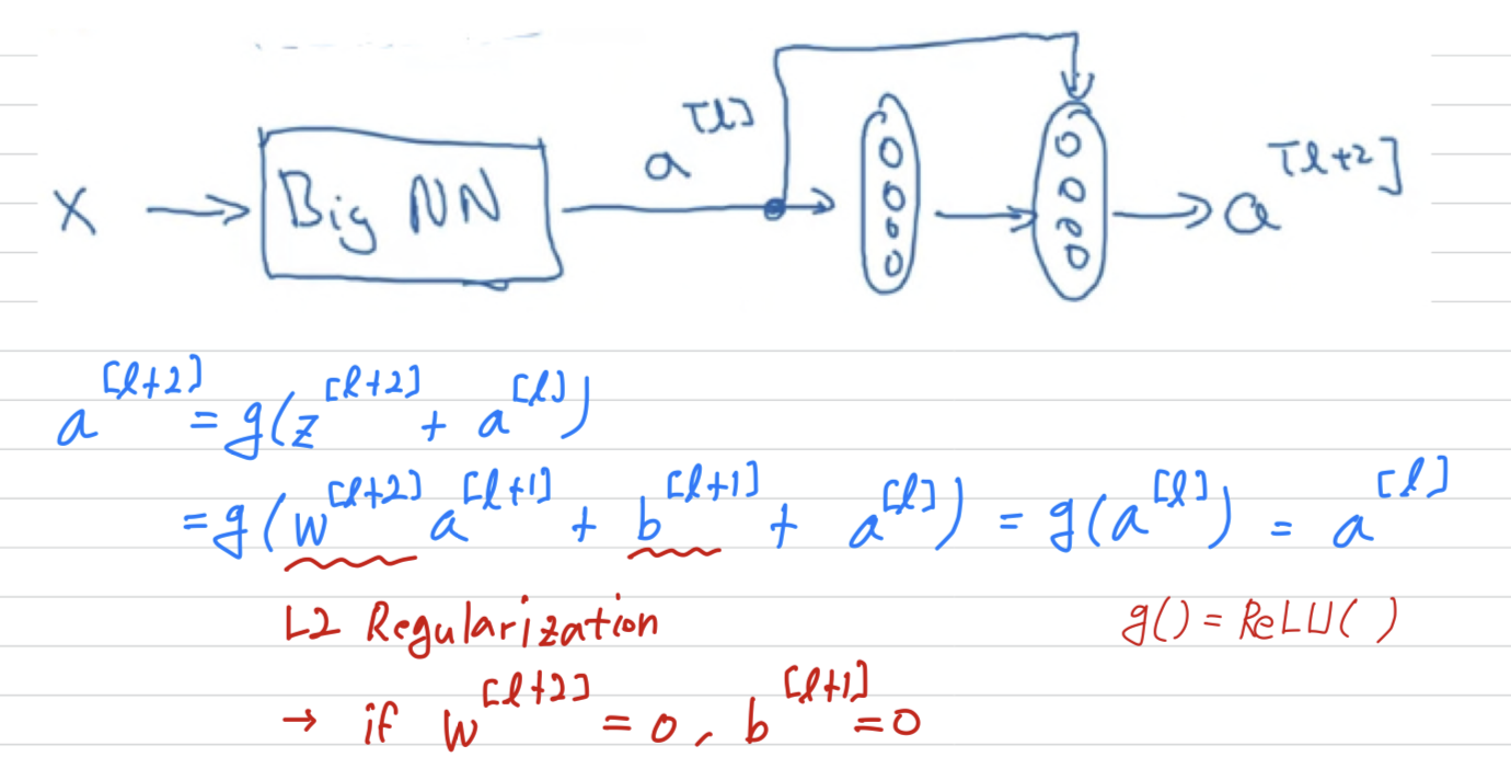  So, what this shows is that the identify function is easy for residual block to learn.
  And what that means is that adding two layers in your neural network,
  it doesn't really hurt your neural network's ability to do as well as this simpler network without these two extra layers,
  because it's quite easy for it to learn the identity function to just copy $a^{[l]}$ to $a^{[l+2]}$ using despite of the addition of these two layers.
  
  But of course our goal is to not just hurt performance,
  and so you can imagine that if all of these hidden units if they actually learned something useful then maybe you can do even better than learning the identity function.
  
  And what goes wrong in very deep plain nets in very deep network without this residual of the skip connections is that when you make the network deeper and deeper,
  it's actually very difficult to for it to choose parameters that learn even the identity function which is why a lot of layers end up making your result worse.
  
  And i think the main reason the residual network works is that
  it's so easy for these extra layers to learn the identity function that you're kind of guaranteed that it doesn't hurt performance and then a lot the time you maybe get lucky and then even helps performance.
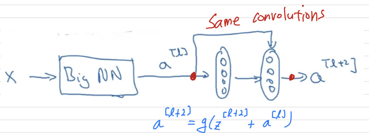  One more detail in the residual network that's worth discussing.
  We're assuming that $z^{[l+2]}$ and $a^{[l]}$ have the same dimension.
  And so what you see in ResNet is a lot of use of same convolutions so that the dimension of $a^{[l]}$ equal to the dimension of $z^{[l+2]}$.
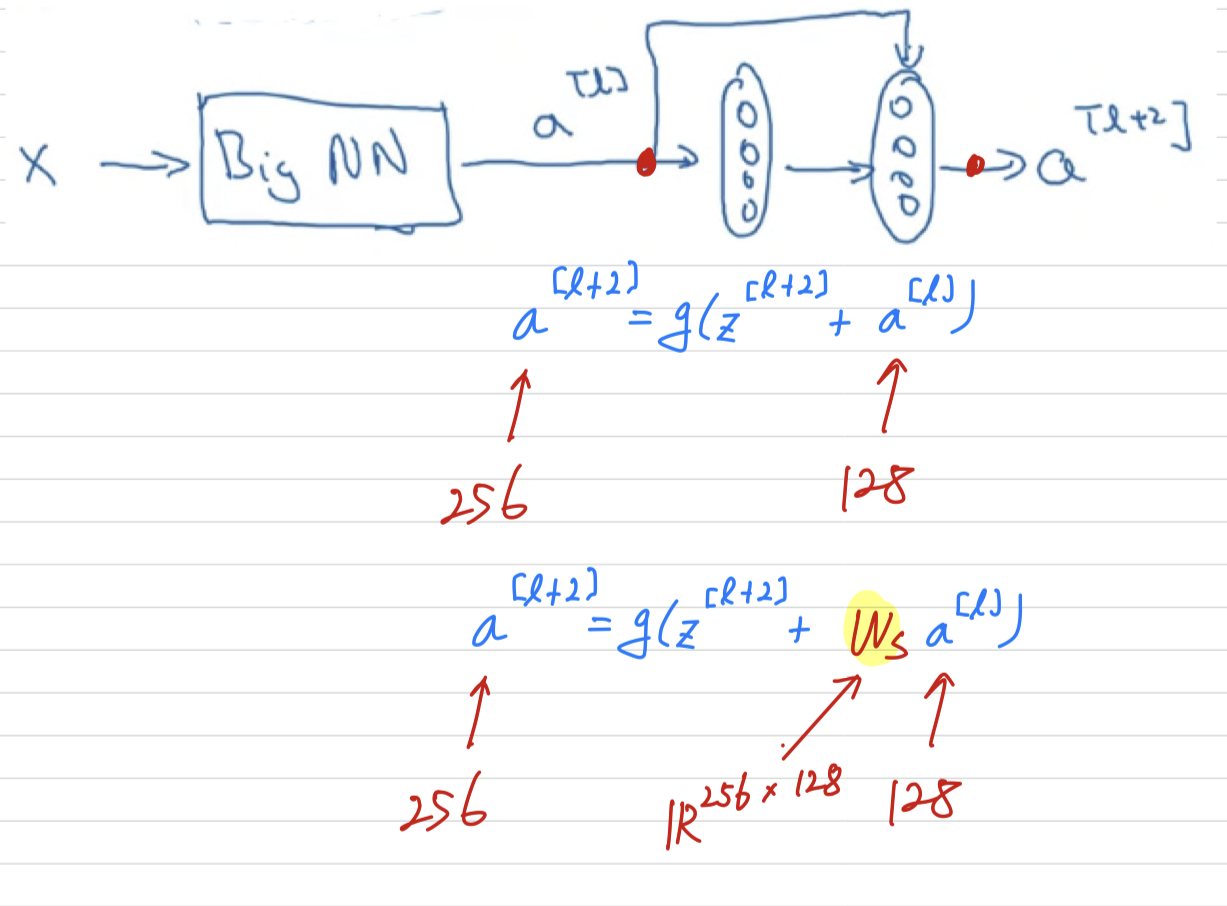  In case the input and output have different dimensions,
  what you would do is add an extra matrix and then call that $W_s$ over there.
  (1) It could be a matrix of parameters we learned.
  (2) It could be a fixed matrix that just implements zero paddings that takes $a^{[l]}$.
  And either of those versions i guess could work.

ResNet

• So these are images i got from the paper by Harlow.
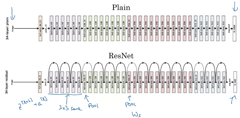  This is an example of a plain network and in which you input an image and then have a number of conv layers until eventually you have a softmax output at the end.
  
  To turn this into a ResNet, you add those extra skip connections.
  There are a lot of $3 * 3$ same convolutions here
  and that' why you're adding equal dimension feature vectors.
  Because these are actually the same convolutions, the dimensions are preserved and so the $z^{[l+2]} + a^{[l]}$ by addition makes sense.
  
  And similar to what you've seen in a lot of network before,
  you have a bunch of convolutional layers and then there are occasionally pooling layers as well.
  And whenever one of those these happens, then you need to make an adjustment to the dimension which we saw on the previous slide.
  You can do of the matrix $W_s$.
  And then as is common in these networks,
  you have Conv Conv Conv Pool, Conv Conv Conv Pool, Conv Conv Conv Pool, ..., FC, Softmax

---

Networks in Networks and 1x1 Convolutions

Why does 1x1 convolution do?

• Here' a $1 * 1$ filter.
  A convolution by $1 * 1$ filter doesn't seem particularly useful.
  You just multiply it by some number.
  But that's the case of $6 * 6 * 1$ channel images.
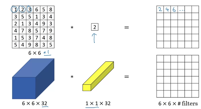  If you have $6 * 6 * 32$ insteand of $6 * 6 * 1$
  then a convolution with $1 * 1$ filter can do something that makes much more sense.
  In particular, what a $1 * 1$ convolution will do is it will look at each of the $36$ different positions here.
  It will take the element-wise product between $32$ numbers on the left and the $32$ numbers in the filter, and then apply a ReLU.
  To look at one of the $36$ positions, maybe one slice through this volume,
  you take these $36$ numbers, multiply it by $1 * 1$ slice through the volume like that and you end up with a single real number.More generally, if you have not just one filter, but if you have multiple filters,
  then it's as if you have no just one unit, but multiple units to taking as input all the numbers in one slice and then building them up into an output, the $(6 * 6 *$ #$filters)$
  
  One way to think about a $1 * 1$ convolution is that it is basically having a fully connected neural network that applies to each of the $62$ different positions.
  What that fully connected neural network does is it $32$ ➡️ $n_C^{[l+1]}$.
  This idea is often called a one-by-one convolution,
  but it's sometimes also called network in network.

Using 1x1 convolutions

• But to give you an example of where 1x1 convolution is useful,
  here's something you could do with it.
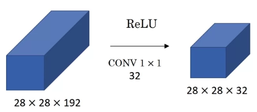  If you want to shrink the height and width, you can use a pooling layer.
  But what about the number of channels has gotten too big and you want to shrink that(192 ➡️ 32).
  What you can do is use, $32$ filters that are 1x1, and technically each filter would be of dimension 1x1x192
  But you use 32 filters and the output of this process will be 28x28x32 volume.
  This is a way to let your strength $n_C$ as well.
  Whereas pooling layer are used just to shrink $n_H, n_W$.
  
  We'll see later how this idea of 1x1 convolutionss allows you to shrink the number of channels and therefore save on computation in some networks.
  But of course, if you want to keep the number of channels to the 192, that's fine too.
  The effect of 1x1 convolution is just has nonlinearity.
  It allows you to learn a more complex function of your network by adding another layer,
  the inputs 28x28x192 and outputs 28x28x192.
  
  You've now seen how a 1x1 convolution operation is actually doing a pretty non-trivial operation
  and allows you to shrink the number of channels in your volumes or keep it the same or even increase it if you want.

---

Inception Network Motivation

Motivation for inception network

• What an inception layer says is,
  instead of choosing what filter size you want in a Conv layer,
  or even do you want a convolutional layer on a pooling layer?
  Let's do them all.
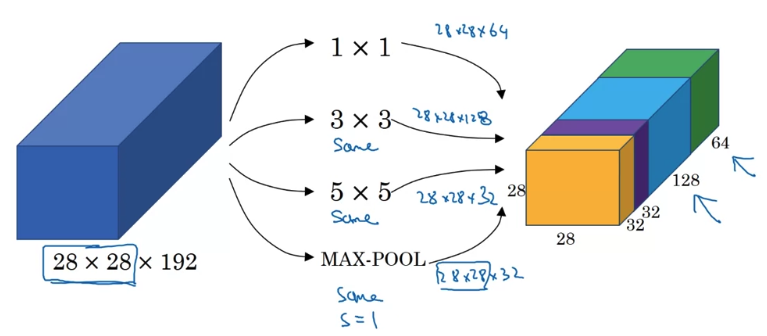  So what if you can use 1x1 convolution,
  Let's say 28 x 28 x 64 output,
  
  But maybe you also want to try a 3 x 3 and that might output a 28 x 28 x 128.
  And then what you do is just stack up this second volume next to the first volume.
  And to make the diimensions match up, let's make this a same convolution.
  So the output dimension is still 28 x 28, same as the input dimension in terms of height and width.
  
  Maybe a 5 x 5 filter works better, so let's do that too and have that output 28 x 28 x 32.
  And again you use the same convolution to keep the dimensions the same.
  And maybe you don't want to convolutional layer.
  
  Let's apply pooling, and that has some other output and let's stack that up as well.
  And here pooling outputs 28 x 28 x 32.
  Now in order to make all the dimensions match,
  you actually need to use padding for max pooling.
  So this is an unusual formal pooling because if you want the input to have a higher than 28 x 28 and have the output, you'll match the dimension everything else also by 28 x 28, then you need to use the same padding as well as $s=1$ for pooling.
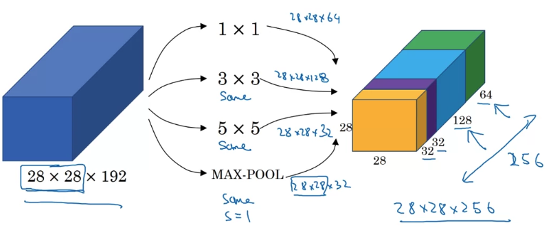  But with a inception module like this,
  you can input some volume and output in this case if you add up all these numbers, $32 + 32 + 128 + 64 = 256$,
  So you will have one inception module input 28 x 28 x 192, and output 28 x 28 x 256.
  
  And this is the heart of the inception network.
  And the basic idea is that instead of you needing to pick one of these filter sizes or pooling you want and committing to that,
  you can do them all and just concatenate all the outputs, and let the network learn whatever parameters it wants to use, whatever the combinations of these filter sizes it wants.
  
  Now it turns out that there is a problem with the inception layer as we've described it here, which is computational cost.
  Let's figure out what's the computational cost of this 5 x 5 filter resulting in this block.

The problem of computational cost

• So just focusing 5 x 5 pot on the previous slide.
  So i'm just going draw this as a more normal looking blue block.
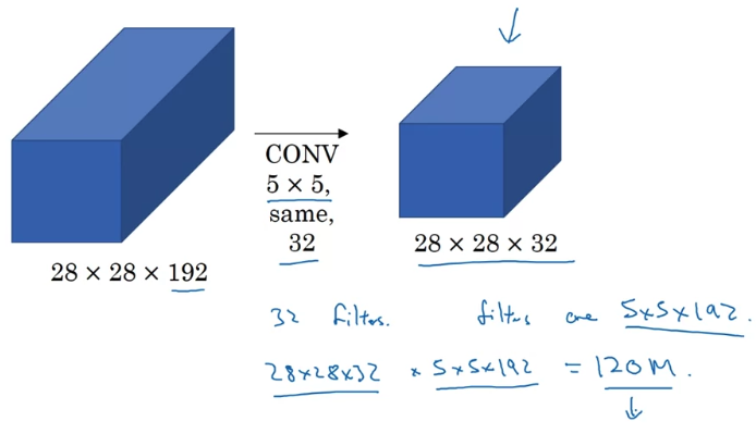  You have 32 filters because the outputs has 32 channels, and each filter is going to be 5 x 5 x 192.
  And so the output size is 28 x 28 x 32, and so you need to compute (28 x 28 x 32) numbers.
  And for each of them, you need to do (5 x 5 x 192) multiplications.
  So the total number of multiplies you need is the number of multiplies you eed to compute each of the output values(5 x 5 x 192) times the number of output values(28 x 28 x 32) you need to compute.
  And if you multiply all of these numbers, this is equal to $120 Million$.
  This is still a pretty expensive operation.
  
  On the next slide, you see how using the idea of 1 x 1 convolutions,
  you'll be able to reduce the computational costs by about $1,200,000 * \frac{1}{10}$.

Using 1x1 convolution

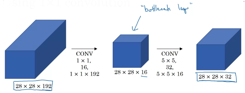• You're going to input the volume, use a 1 x 1 convolution to reduce the volume to 16 channels instead of 192 channels,
  and then on this much smaller volume,
  run your 5 x 5 convolution to give you final output.
  So notice that input and output dimensions are still the same as previous slide.
  But what we've done is we're taking this huge volume(28 x 28 x 192) we had on the left,
  and we shrunk it to this much smaller intermediate volume, which is only has 16 instead of 192 channels.
  Some time this is called a bottleneck layer.
  The bottleneck is the smallest part of this bottle.
  So in the same say, the bottleneck layer is the smallest part of this network.
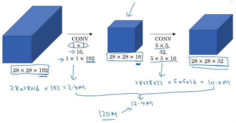  The total number of multiplications you need to do is the sum of those which is $12.4 Million$.
  And you compare this with what we had on the previous slide,
  you reduce the computational cost from about $120 Millon$ multiplies down to about $\frac{1}{10}$ of that.

So to summarize, if you are building a layer of a neural network and you don't wantt to have to decide, do you want a 1 x 1, or 3 x 3, or 5 x 5, or pooling layer, the inception module
let's do them all, and let's concatenate the results.

And then we run to the problem of computational cost.
And what you saw was how using a 1 x 1 convolution,
you can create this bottleneck layer thereby reducing the computational cost significantly.

Now you might be wondering, does shrinking down the representation size so dramatically,
does it hurt the performance of your neural network?
It turns out that so long as you implement this bottleneck layer so that within reason,
you can shrink down the representation size significantly, and it doesn't seem to hurt the performance, but saves you a lot of computation.

So these are the keys ideas of the inception module.
Let's put them together and show you waht the full inception network looks like.

---

Inception network

• You've already seen all the basic building blocks of the Inception network.
  In this video, let's see how you can put these building blocks together to build your own Inception network.
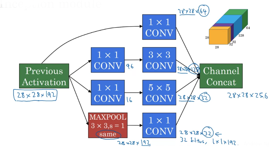  In order to really concatenate all of these outputs at the end
  we are going to use the same type of padding for pooling.
  But notice that if you do Max Pooling even with same padding, the output wil l be 28 x 28 x 192.
  It will have the same number of channels and the same depth as the input.
  So this seems like is has a lot of channels.
  So what we're going to do is actually add one more 1 x 1 conv layer to strengthen the number of channels.
  So it gets us down to 28 x 28 x 32.
  And the way you do that, is to use 32 filters of dimension 1 x 1 x 192.
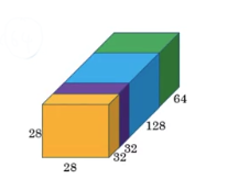  And finally you take all of these blocks and you do channel concatenation.
  Just concatenate across 64 + 128 + 32 + 32 = 256,
  this if you add it up this gives you a 28 x 28 x 256 dimension output.
  
  So this is one inception module, and what the inception network does is
  more or less put a lot of these modules together.

• Here's a picture of the inception network, taken from the paper by Szegedy et al.And you notice a lot of repeated blocks in this.
  Maybe this picture looks really complicated.
  But if you look at one of the blocks there, that block is basically the inception module that you saw on the previous slide.
  
  And subject to little details i won't discuss,
  There is another inception blocks.
  There's some extra max pooling layers to change the dimension of the height and width
  but bascially there's another inception block.Which is that are these additional side-branches.
  So what do tey do?
  The last few layers of the network is a fully connected layer followed by a softmax layer to try to make a prediction.
  What these side branches do is it takes some hidden layer and it tries to use that to make a prediction.
  So this is actually a softmax output.
  And this other side branch again it is a hidden layer passes through a few layers like a fully connected layers.
  And then has the softmax try to predict what's the output label.
  
  What is does is it helps to ensure that the features computed, even in the hidden units.
  That they're not too bad for protecting the output cause of a image.
  And this appears to have a regularizing effect on the inception network and helps prevent this network from overfitting.
  
  Where does the name inception come from?
  If you've seen the movie title The Inception, maybe this meme("We need to go deeper") will make sense to you.
  But the authors actually cite this meme as motivation for needing to build deeper neural networks.
  And that's how they came up with the inception architecture.

---

MobileNet

• In this video, you'll learn about MobileNet, which is another foundational convolutional neural nework architecture used for computer vision.
  Using MobileNet will allow you to build and deploy neural networks that work even in low compute environment such as mobile phone.

Motivation for MobileNets

• Why do you need another neural network architecture?

  • Low computational cost at deployment :
    It turns out in other neural networks you've learned about so far qre quite computationally expensive.
    If you want your neural network to run on a device with less powerful CPU or GPU at deployment, then there's another neural network architecture called the MobileNet that could perform much better.
  • Useful for mobile and embedded vision applications

• Key idea : Normal vs depthwise-separable convolutions

Normal Convolution

• In the normal convolution,
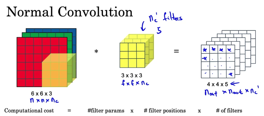
  Let's figure out what is the computational cost of what we justied.
  It turns out the total number of computations needed to compute this output is given

Depthwise Separable Convolution

• Let's see how the separable convolution does that.
  In contrast to the normal convolution, the depthwise separable convolution has two steps.
  You're going to first use a depthwise convolution, follwed by a pointwise convolution.
  These two steps which together make up depthwise separable convolution.

1. Depthwise Convolution
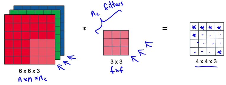   Let's focus on just the red one.
   And carry out the 9 multiplications not 27, and add them up.
   
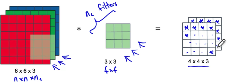
   Next we go to the second channel.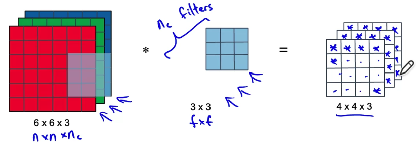Finally we do this for the third channel.
   
   The size of output after this step will $(n_{out} * n_{out} * n_C)$
   ($n_C$ is the same as the number of channels in your original input)
   
   Let's look at the computational cost of what we've just done.
   
   We're not yet done.
   This is a depth-wise convolution part of the depth wise separable convolution.
   There's one more step,
   which is we need to take this (4 x 4 x 3) intermidiate value and carry out one more step.

2. The remaining step is to take this (4 x 4 x 3) set of values, or $(n_{out} * n_{out} * n_C)$ set of values,
   and apply a pointwise convolution in order to get the output we want which will be (4 x 4 x 5).
   Let's see how the pointwise convolution works.
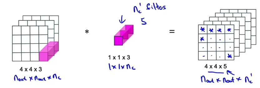   Here's the pointwise convolution.
   We are going to take the intermediate set of values, which is $(n_{out} * n_{out} * n_C)$
   and convolve it with a filter that is $(1 * 1 * n_C)$.The total cost of what we just did here is $240$ multiplications.

• In the example we just walked through,
  the normal convolutoin,
  took as input a $6 * 6 * 3$ input, and wound up with a $4 * 4 * 5$ output.
  And same for the depthwise separable convolution, except we did it in two steps
  with a depthwise convolution, followed by a pointwise convolution.

• Now, What were the computational costs of all of these operations?
  

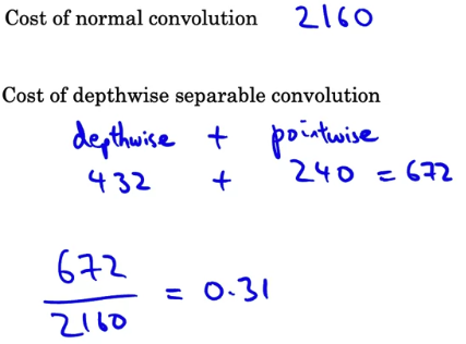
  • In the case of the normal convolution,
    we needed $2160$ multiplications to compute the output.
  • For the depthwise separable convolution,
    there was first step the depthwise step, where we had $432$ multiplications
    and then the pointwise step, where we had $240$ multiplications
    and so adding these up, $672$ multiplications.
    
    If we look the ratio between these two numbers, $\frac{672}{2160}=0.31$.
    In this example, the depthwise seaparable convolution was about $31$ percent as computationally expensive as the normal convolution.
    
    The authors of the MobileNets paper showed that in general,
    the ratio of the cost of the depthwise separable convolution compared to the normal convolution,
    that turns out to be $\frac{1}{n_C'} + \frac{1}{f^2}$.
    In our case, this was $\frac{1}{5} + \frac{1}{3^2} \simeq 0.31$
    
    In a more typical neural network example, $n_C'$ wil be much bigger.
    So it maybe, say, $\frac{1}{512} + \frac{1}{3^2}$.(This would be a fairly typical parameters of neural network)
    So very roughly, the depthwise separable convolution may be
    about $\frac{1}{9}$ rounding up roughly $10$ times cheaper in computational costs.
    
    That's why the depthwise separable convolution as a building block of a convnet,
    allows you to carry out inference much more efficiently than using a normal convolution.

---

MobileNet Architecture

• In the last video you learned about the depthwise separable convolution.
  Let's now put this into a neural network in order to build the MobileNet.

• You can now instead use a much less expensive depthwise separable convolutional operation,
  comprising the depthwise convolution operation.
  The MobileNet v1 paper had a speicific architecture in which it use a block $13$ times.
  So it would use a depthwise convolutional operation to genuine outputs
  and then have a stack of $13$ of these layers in order to go from the original raw input image to finally making a classification prediction.
  
  Just to provivde a few more details after these $13$ layers,
  the neural networks last few layers are the usual Pooling layer, followed by a fully connected layer, followed by a Softmax in order for it to make a classification prediction.
  
  This turns out to perform well while being much less computationally expensive than earlier algorithms that used a normal convolutional operation.
  
  I want to share with you one more improvement on this basic MobileNet architecture, which is the MobileNets v2 architecture.
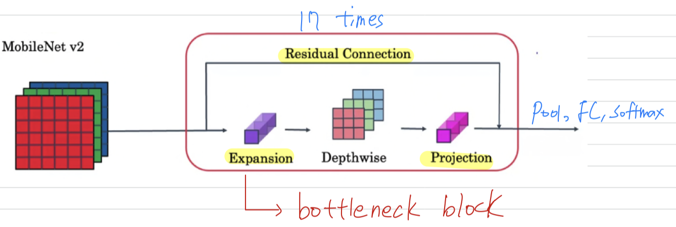  In MobileNet v2, there are two main changes.
  
  One is the addition of a residual connection.
  This residual connection or skip connection takes the input from the previous layer and sums it or passes it directly to the next layer,
  does allow gradient descent, propagate backward more efficiently.
  
  The second change is that it also as an expansion layer,
  which you learn more about on the next slide, before the depthwise convolution, followed by the pointwise convolution, which we're going to call Projection in a point-wise convolution is really the same operation, but we'll give it a different name, for reasons that you see on the next slide.
  
  The MobileNet v2 architecture happened to choose to $17$ times,
  so pass the inputs through $17$ of these blocks,
  and then finally ends up with usual pooling, fully-connected, softmax in order for it to make a classification prediction.
  
  But the key idea is really how blocks reduces computational cost.
  This block is also called the bottleneck block.

MobileNet v2 Bottleneck

• Let's dig into the details of how the MobileNet v2 block works.
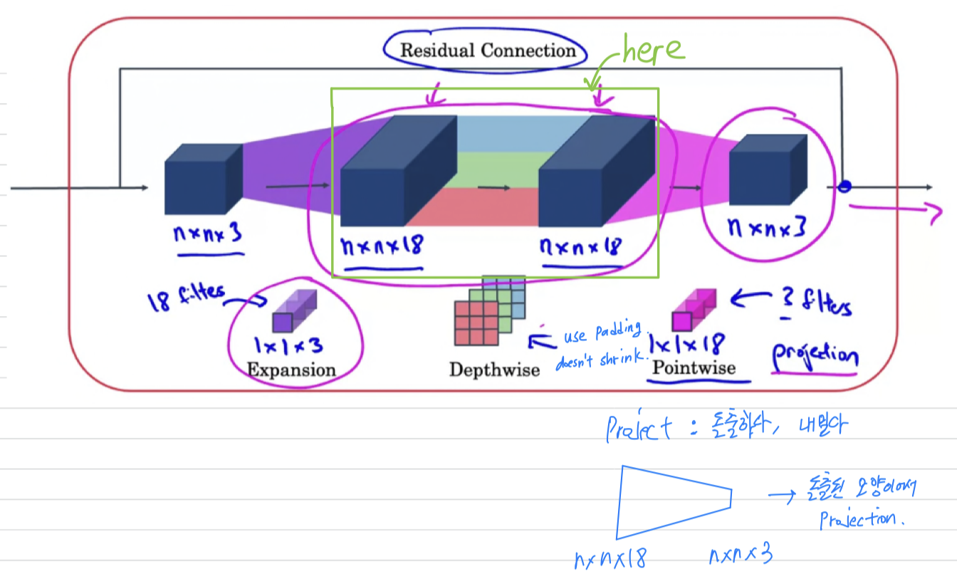  So you might be wondering, why do we need these bottleneck blocks?
  ➡️ It turns out that the bottleneck block accomplishes two things.
  One, by using the expansion operation,
  it increases the size of the representation within the bottleneck block.
  This allows the neural network to learn a richer function.
  There's just more computation over here.
  But when deploying on a mobile device, on edge device,
  you will often be heavy memory constraints.
  And so the bottleneck block uses the pointwise convolution or the projection operation in order to project it back down to a smaller set of values,
  so that when you pass this the next block,
  the amount of memory needed to store these values is reduced back down.
  
  So the clever idea, the cool thing about the bottleneck block is that
  it enables a richer set of computations, thus allow your neural network to learn richer and more complex functions, while also keeping the amounts of memory that is the size of the activations you need to pass from layer to layer, relatively small.
  That's why the MobileNet v2 can get better performance than MobileNet v1,
  while still continuing to use only a modest amount of compute and memory resoureces.

---

EfficientNet

• MobileNet V1 and V2 gave you a way to implement a neural network, that is more computationally efficient.
  But is there a way to tune MobileNet, or some other architecture, to your specific device?
  How can you automatically scale up or down neural networks for a paticular device?
  EfficientNet, gives you a way to do so.
  
  Let's say you have a baseline neural network architecture,
  where the input image has a certain resolution $r$
  and your neural network has a certain $d$ = depth, and the layers has a certain $w$ = width.
  
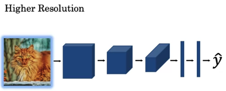
  The authors of the EfficientNet paper observed that the three things you could do to scale things up or down.

1. you could use a high resolution image.
   

2. you could make this network deeper.
   so you could vary $d$ to depth of the neural network,
   

3. you could make this network wider.
   so you could vary $w$ to width of the neural network,
   

The question is,
given a particular computational budget, what's the good choice of $r, d$ and $w$?
Or depending on the computational resources you have,
you can also use compund scaling, where you might simultaneously scale up or simultaneously scale down the resolution of the image,

Now the tricky part is,
if you want to scale up $r, d$ and $w$, which you should scale up each of these?
What's the best trade-off between $r, d$ and $w$ to sacle up or down your neural network,
to get the best possible performance within your computational budget?

So if you are ever looking to adapt a neural network architecture for a particular device,
look at one of the open source implementations of EfficientNet,
which will help you to choose a good trade-off between $r, h$ and $w$.

---

Seminar - discussion

• x가 jump해서 $f(x)+x$로 된다.
  기존에는 network가 깊어질수록 gradient가 0이 될 수 있는 vanishing문제가 발생했다.
  그래서 Batch Normalization으로 많이 해결했었지만 그래도 network가 너무 길면, vanishing 문제가 생길 수도 있다.
  그래서 중간중간에 layer를 skip하여 activation 값을 더해주자.
  입력이 거의 살아서 마지막까지 갈 수 있다.
  반대로 backprop에서 끝에서 수행한 gradient도 처음 부분까지 살아서 갈 가능성이 있다.
  입력값과 backprop에서 gradient값을 마지막까지 전달되는 확률을 높이겠다는 것이 아이디어였다.
  즉, 너무 깊어지면 소실되는 정보를 살리려는 목적.
  
  $F(x)$를 residual function이라고 한다.
  만약 skip path가 없다고 하면, $x$가 2번 변하여 나온 결과인 $F(x)$에 대해서 학습하기 위해 다음 Layer에서는 힘들어질 것이다.
  그래서 원래 있던 $x$값에서 약간 변화시켜서 (2 layer만큼 변화) 그 변화값 $F(x)$에 $x$를 더해준다.
  그래서 2개의 layer는 복잡한 학습을 하는 것이 아니라 더 편하게 학습을 할 수 있을 것이다.
  $x$가 보존이 되어있기 때문에 residual function은 $x$에서 변환되는 작은 양만 배울 수 있기 때문에 학습이 훨씬 빠르고 수월할 것이다.
  즉, 원래 것에서 첨가되는 나머지의 것을 배우겠다는 것.
  
  시간이 중요한게 아니라 정확도가 중요한 경우,
  앙상블 networksms network 1, 2, 3, ..., 10 의 후보들을 동시에 학습시켜서 그 중 높은 성능을 얻어내는 networkdlek.
  skip을 시키면, 여러 sub network가 생긴다.
  residual network는 많은 subnetwork가 들어있는 것이라, 앙상블 network와 같은 비슷한 효과를 낼 수 있다는 말도 있다.

• 논문들 중에서는 (1) 수학적으로 증명 또는 (2) 실험적인 평가 데이터 둘 중 하나만이 있는 논문들이 있다.
  ResNet같은 경우는 수학적으로 완전히 증명되어 왜 network가 잘 되는지는 안나와있다.
  여러 평가 데이터를 통해 ResNet이 잘 되었다는 것이다.

• CNN에서 data는 모두 augmentation을 한다.
  Random Cropping, Random Mirroring은 무조건 하는 augmentation이다.
  똑같은 하나의 Image를 100번 random cropping을 하면, 조금이라도 다르니까 100개의 서로 다른 image가 된다.
  설령 data가 많더라도 augmentation은 무조건 한다.
  능을 많이 향상시킬 수 있다.