Clustering : Introduction

Clustering is

• data segmentation
• grouping

such that those within each cluster are more closely related to one another than objects in others. Note that clustering

• is $unsupervised$, which means there is no right answer to learn
• the definition of $similarity$ (or $distance$, in the same meaning) is important (and subjective)

In this post, we will explore the followings:

• Generate a toy dataset for clustering
• Do cluster anlaysis on the dataset and visuakuzed this:
  • K-means
  • Gaussian mixture
  • Hierachical clustering
  • Self-Organizing Map
  • Spectral clustering
• Evaluate clustering results

---

Settings in python

Libraries

Bring your packages to do cluster analysis and make plots in python:

import pandas as pd
import numpy as np
import math
import scipy as sp

import matplotlib.pyplot as plt

Example data generation

To make a toy example data set, make_blobs in sklearn.datasets is used

• make_blobs generate $isotropic$ $Gaussian$ blobs for clustering
  • which means whose covariance is simplified as $\Sigma=\sigma^2 I$
• you can change the argument random_state and choose an appropriate
  • my choice is 7
• For more detailed information, visit here

from sklearn.datasets import make_blobs

x, y = make_blobs(n_samples=100, centers=3, n_features=2, random_state=7)
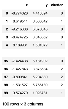
points = pd.DataFrame(x, y).reset_index(drop=True)
points.columns = ["x", "y"]
points.head()

Check your generated toy using plot below: It is so pretty!

• As you may have already noticed, the number of clusters is 3

import seaborn as sns
sns.scatterplot(x="x", y="y", data=points, palette="Set2");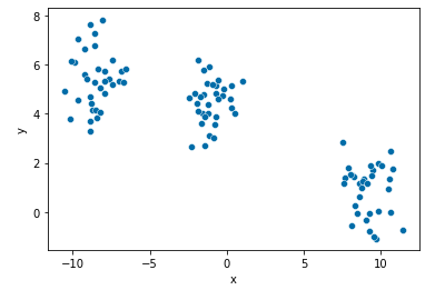

Color map

For a pretty visualization, I'd like to have three color palettes in advance:

import matplotlib.pyplot as plt

def get_cmap(n, name='viridis'):
    '''Returns a function that maps each index in 0, 1, ..., n-1 to a distinct 
    RGB color; the keyword argument name must be a standard mpl colormap name.'''
    return plt.cm.get_cmap(name, n)

cmap = get_cmap(3)

---

Clustering algorithms

1. K-means

The $K$-$means$ clustering is

• the most popular iterative descent clustering methods
  • $iterative$ $greedy$ $descent$ : identify a small subset that is likley to contain the optimal one, or at least a good suboptimal partition

A practical issue of K-means clustering on initial values:

• should start the algorithm with many different random choices for the starting means
• and choose the solution having smallest value of the objective function

• Fitting model

from sklearn.cluster import KMeans

model = KMeans(n_clusters = 3, random_state = 10)
model.fit(points)
kmeans_labels = model.fit_predict(points)
points['cluster'] = kmeans_labels

• Plotting

import matplotlib.pyplot as plt

fig = plt.figure()
for i in range(len(points)):
    plt.plot([points['x'][i]], [points['y'][i]], marker='o', color=cmap(points['cluster'][i]))

---

2. Gaussian mixture

The $K$-$means$ clustering procedure is closely related to the $EM$ algorithm for estimating a certain Gaussian mixture model

• K-means : deterministic
• Gaussian mixture : probabilistic
  • They use concept the $relative$ $densities$, using normal distribution centered on each centroid
    

For more on clustering using Gaussian mixture, go to here.

• Fitting model

from sklearn.mixture import GaussianMixture

gmm = GaussianMixture(n_components=3, random_state=42)
gmm_labels = gmm.fit_predict(points)

points['cluster'] = gmm_labels

• Plotting

import matplotlib.pyplot as plt

fig = plt.figure()
for i in range(len(points)):
    plt.plot([points['x'][i]], [points['y'][i]], marker='o', color=cmap(points['cluster'][i]))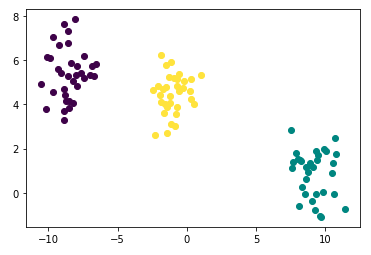

---

3. Hierachical clustering

$K$-$means$ clustering algorithm depends on

• the choice for the number of clusters
• a (random) starting configuration assignment

In contrast, $hierachical$ $clustering$ methods do not require such specifications. Instead, they require

• a measure of dissimilarity between disjoint $groups$ of obsevations

Strategies for hierachical clustering divide into two basic paradigms:

• agglomerative (bottom-up) - mostly used
• divise (top-down)

For more detailed description, you can see this.

• Dendrogram

import scipy.cluster.hierarchy as shc

plt.figure(figsize=(10, 6))
plt.title("Customer Dendograms")
dend = shc.dendrogram(shc.linkage(points, method='ward'))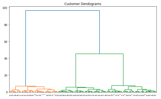

• Fitting model

from sklearn.cluster import AgglomerativeClustering

hierachical_fit = AgglomerativeClustering(n_clusters=3, affinity='euclidean', linkage='ward')
hac_labels = hierachical_fit.fit_predict(points)

points['cluster'] = hac_labels

• Plotting

import matplotlib.pyplot as plt

fig = plt.figure()
for i in range(len(points)):
    plt.plot([points['x'][i]], [points['y'][i]], marker='o', color=cmap(points['cluster'][i]))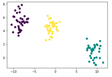

---

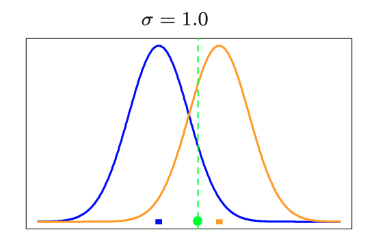
4. Self-Organizing Maps

The Self-Organizing Maps(SOM) procedure

• can be viewed as a constrained version of $K$-$means$ $clustering$
• tries to bend the plane so that the buttons(green dots) approximate the data points as well as possible

The original SOM algorithm was $online$

• i.e., observations are processed one at a time
• Later, a batch version was proposed

Begin $SOM$ in Python! Package minisom do this.

• Data processing
  • Note that function MiniSom requires data in array form, not in dataframe

points_dataset = []
for i in range(points.shape[0]):
    point_series = np.array(points.iloc[i,:])
    points_dataset.append(point_series)

• Fitting model

from minisom import MiniSom
som = MiniSom(3, 1, # initialization of 3x3 SOM
              len(points_dataset[0]), # length of dataset
              sigma=0.3,
              learning_rate = 0.1)
som.random_weights_init(points_dataset)
som.train(points_dataset, 1000)
win_map = som.win_map(points_dataset)

• Plotting

import matplotlib.pyplot as plt

fig = plt.figure()
for i, (x, y) in enumerate(points_dataset):
    fitted_ = som.winner(points_dataset[i])
    cluster_number = (fitted_[0] * 1) + fitted_[1]
    plt.plot([x], [y], marker='o', color=cmap(cluster_number))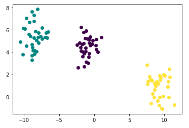

---

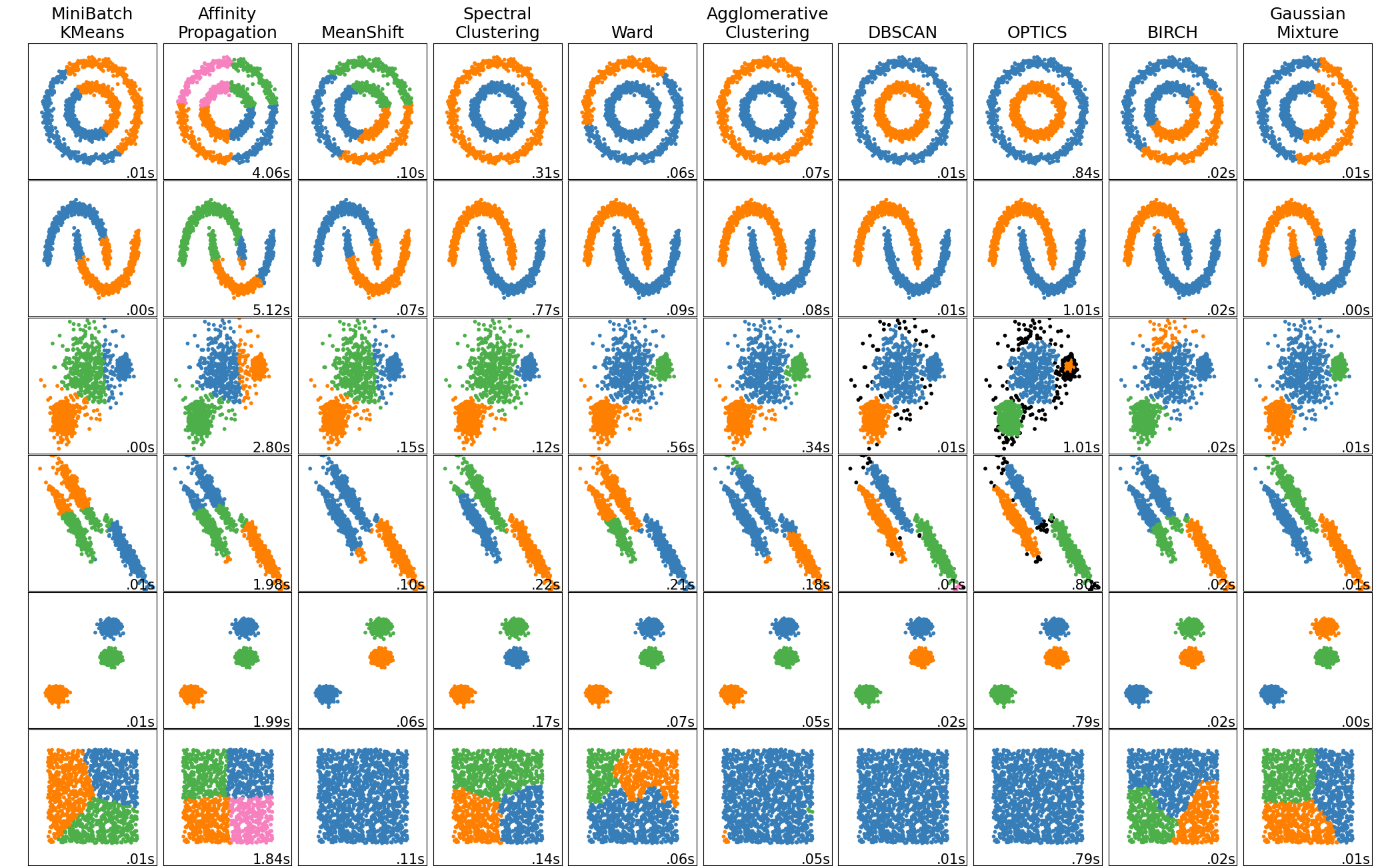
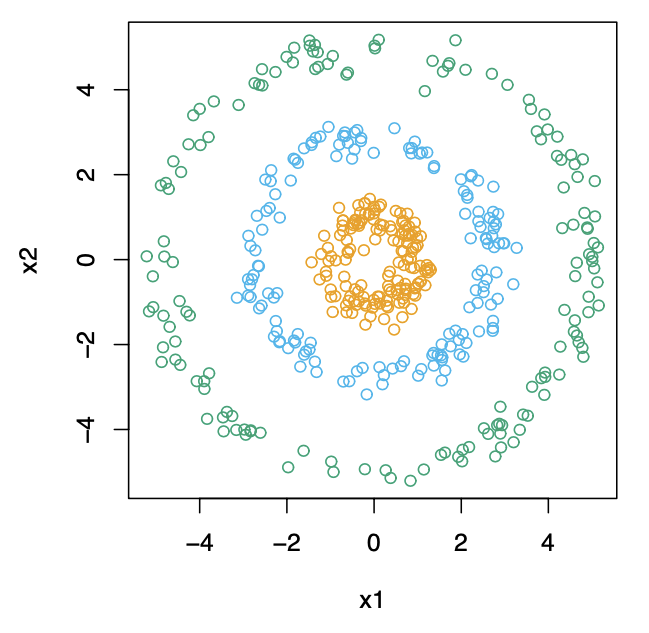
5. Spectral clustering

Traditional clustering method like K-means

• use a spherical or elliptical metric to group data points
• they will not work well for the other shape of clusters

$Spectral$ $clustering$ is designed for

• the non-convex shape clusters, such as the concentric circles as below
• For detailed illustration, visit are here!
  

• Fitting model

from sklearn.cluster import SpectralClustering
sc = SpectralClustering(n_clusters=3).fit(points)
sc_labels = sc.labels_

points['cluster'] = sc_labels

• Plotting

import matplotlib.pyplot as plt

fig = plt.figure()
for i in range(len(points)):
    plt.plot([points['x'][i]], [points['y'][i]], marker='o', color=cmap(points['cluster'][i]))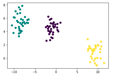

---

Performance evaluation

Clustering is the most representative $unsupervised$ $learning$

• $unsupervised$ means that the algorithm has no right answer to learn
• and also evaluating the algorithm is not a simple matter

For clustering, there are two types of evaluation criteria

• depending on whether they have a cluster label that is the correct answer or not
• Here, we assume that there is NO absolute right label for data
• For more description on clustering performace evaluation in python, go to here

Before compute out evaluation scores, we import metric from sklearn

from sklearn import metrics

Also, our dataset points is a pd.DataFrame like below

• Silhouette Coefficient

from sklearn import metrics
metrics.silhouette_score(points[["x", "y"]], np.ravel(points[["cluster"]]))

• Calinski-Harabasz Index

from sklearn import metrics
metrics.silhouette_score(points[["x", "y"]], np.ravel(points[["cluster"]]))

• Davies-Bouldin Index

from sklearn import metrics
metrics.silhouette_score(points[["x", "y"]], np.ravel(points[["cluster"]]))

[References]

• Hastie, T., Tibshirani, R., Friedman, J. (2008) The Elements of Statistical Learning : Data Mining, Inference, and Prediction. Springer
• https://towardsdatascience.com/time-series-clustering-deriving-trends-and-archetypes-from-sequential-data-bb87783312b4
• https://scikit-learn.org/stable/modules/clustering.html#clustering-performance-evaluation