(Franco-Pedroso, J., 2019) Generating Virtual Scenarios of Multivariate Financial Data for Quantitative Trading Applications

이향기·2022년 2월 23일

Franco-Pedroso, J., Gonzalez-Rodriguez, J., Cubero, J., Planas, M., Cobo, R., & Pablos, F. (2019). Generating Virtual Scenarios of Multivariate Financial Data for Quantitative Trading Applications. The Journal of Financial Data Science, 1(2), 55–77.

1 Introduction
2 Assessment of simulated financial time series
3 Evaluation of stochastic models as simulation methods
4 Generation of virtual scenarios for multivariate data
5 Generation of new artificial assets
6 Analysis of long-term high-dimensional virtual scenarios
7 Conclusion and future work

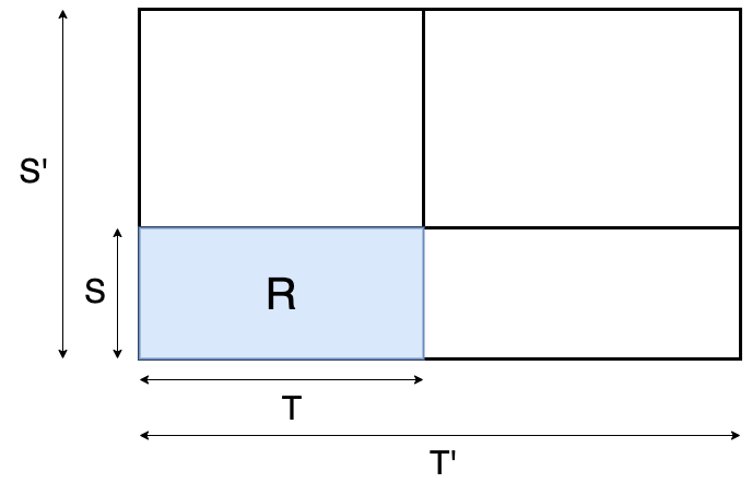
To develop a technique that
- allows to simulate virtual scenario of given financial market
- involving hundres/thousands of assets
- for time period of arbitrary length $VS = f(\mathcal{M}, \mathcal{A}, T)$ where $VS$ : virtual scenario, $\mathcal{M}$ : given financial market, $\mathcal{A}$ : the set of assets and $f$ is a proper function.

Section	Question
2	How to evaluate simulated scenarios?	Just sanity check
3	Limitation of existing models
4	Proposed model to generate virtual scenarios
5	Proposed method to generate artificial assets
6	Sec4+Sec5 and Evalutaion

How to evaluate simulated scenarios?

Assessment of simulated financial time series

Data desciption

Stock prices/returns

Period : 2000/01/01 ~ 2016/04/29
330 stocks in S&P500 index

Market index

Equally weighted

Empirical properties of financial time series

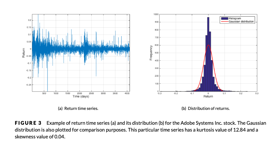
Distributional properties (of asset returns)

shape-piked, fat-tailed : larger kurtosis (> 3)
skewness : individual stock/marker index
rolling metric : time-varying dynamics

Dependency properties

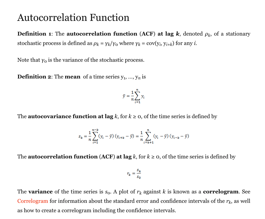
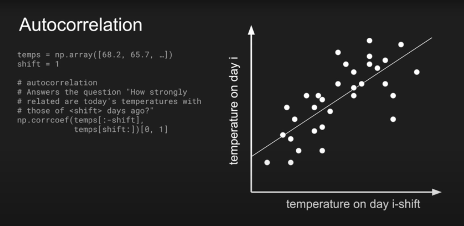
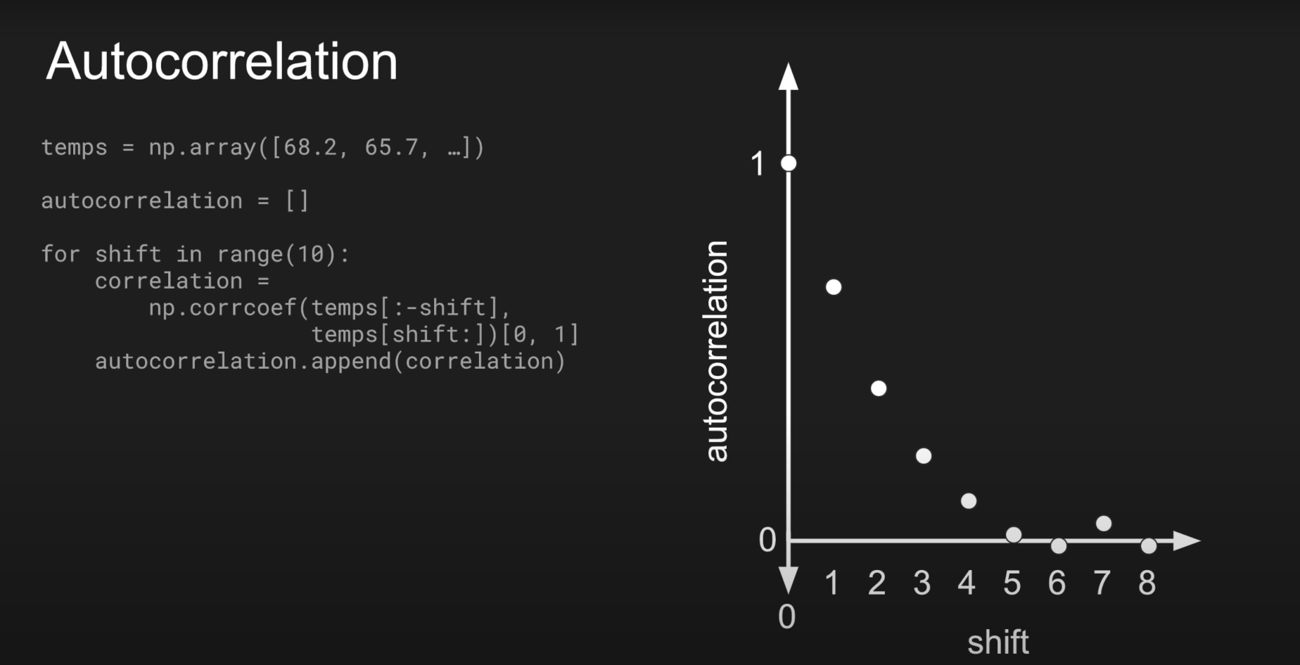
Volatility clustering : ACF(Autocorrelation function) of absolute/squared returns

Pathwise properties

The irregularity of the trajectory

meaused by the number of (linear) trends (segments) over a given time period

Trend ratio

= the return / (the period of the contained trend / the noise level)
= (the return * the noise level) / the period of the contained trend

Cross-asset relationships

Correlation coefficient matrix
What about dynamic behavior? (time-varying)

Number of trends (linear segments) in Market index!
Directional similarity

=the percentage of assets whose prices move in the same direction with market index (within a given direction)
moving average with window size = 50, step size = 1

Financial time series : returns? price?
- Usually, modeling return!
- Because, price is nonnegative
(In 2.1, p.4) How to account for the correlation between assets by market index(=average of assets)?
Can kurtosis grasp shape-pike property of asset dist'n?
Definition of asset return?
Large autocorrelation in large lag value
(In 2.2.3, p.8) What is "the noise level?"

Existing models to generate scenario : Univariate

Stochastic models
- GBM(the Geometric Brownian Motion)
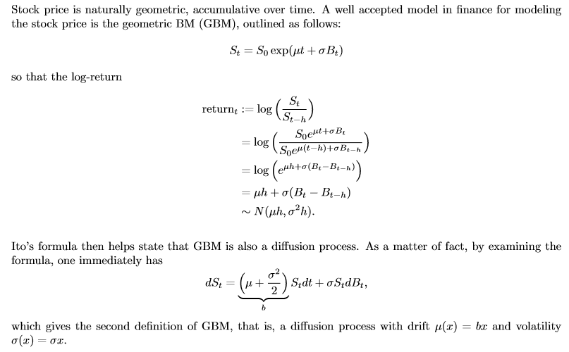
  - fails to reproduce the excess of kurtosis
  - fails to reproduce the volatility clustering feature
Volatility models : ARCH, SV
- Modeling volatility as a time-varying process
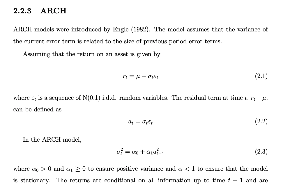
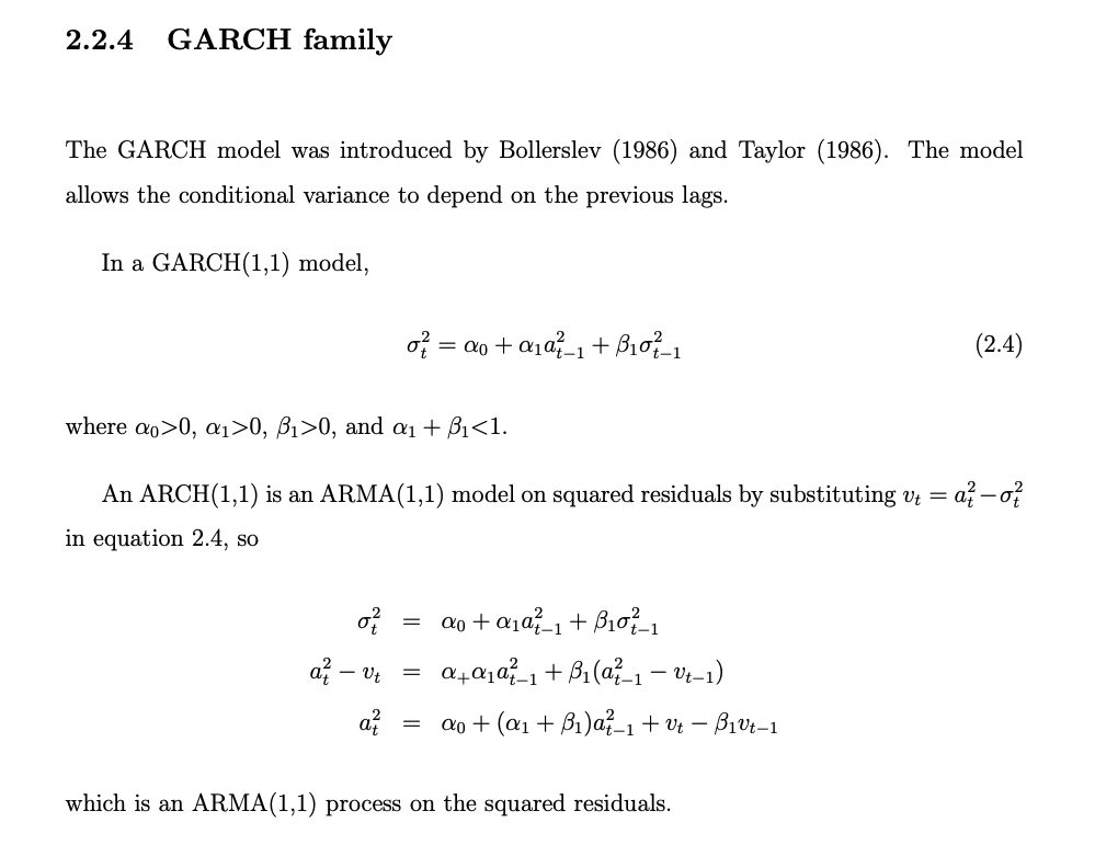
- GARCH : reveals the volatility clustering & the excess kurtosis,
- But when analyzing rolling of them , GARCH model vary at a slower rate that in real stocks -> a different dist'n is needed
- GARCH + Student's t innovation
  - the excess of kurtosis can be better reproduced & the variance of rolling kurtosis value is still low
  - while rolling skewness values vary in a more similar range than that of the real stock

Generation of virtual scenarios for multivariate data

Section4

Stage1) The analysis stage

[Segmentation] Detecting of market trends
- Input : market index (eqally weighted)
- Output : change point, signs
- How:
  - package piecewise_regression
  - package pwlf
- cf. There is any seg method with alternating sign constraint?
[Estimation] Analyzing the multivariate data within each trends to capture both dynamic and statistical properties
- Within segment $s$ , ( $s=1,2,\dots,S)$
  - Let all obeserved return values : $R_{s} = \{r_{\{s,1\}}, r_{\{s,2\}},...,r_{\{s,n(s)\}}\}$
  - The corresponding set in sliding window $w(s)$ :
    $\{r\}_{w(s)}^{L}=\{r_{\{s, t-L/2\}},\dots,r_{\{s, t\}},\dots, r_{\{s, t+L/2\}}\}$
  - What is the step size of sliding window? 1?
- Totally, there are $\sum_{s=1}^{S} W(s)$ normal distributions
- Input : data points {r}_{w(s)}^{L}, sliding window size $L$
- Output : $\{(\hat{\mu_{1}}, \hat{\Sigma_{1}}), (\hat{\mu_{2}}, \hat{\Sigma_{2}}), \dots, (\hat{\mu_{W}}, \hat{\Sigma_{W}})\}$
functions

def mul_normal_est(x, L):
	w = len(x) - L + 1
    for i in range(1, w):
    	# estimate the multivariate normal distribution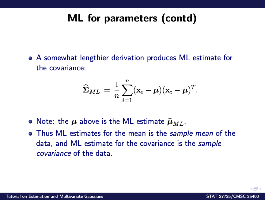
    return mu_list, Sigma_list

Body

market_index = # market index data set (equally weighted)
detected_trends = trend_detection(market_index)
Segments = detected_trends['change_points']

for seg in Segments:
	for win in Windows:
    	mu_hat = # estimation for mu in current sliding windows
        Sigma_hat = # estimation for Sigma in current sliding windows
    	mu_trend = mu_trend.append(mu_hat)
        Sigma_trend = Sigma_trend.append(Sigma_hat)
    mu_total = mu_total.append(mu_trend)
    Sigma_total = Sigma_total.append(Sigma_trend)

Stage2) The synthesis stage

[Hypothesizing] A stochastic sequence of trend is hypothesized
- What hypothesized means in accurate?
- cf. with constraint alternating signs!
[Random generation] For each trend, learned parameters are recovered and multivariate random asset returns are generated for that trend
- Within a given trend, the sequence of $W$ parameters $\{(\mu_{1}, \Sigma_{1}), (\mu_{2}, \Sigma_{2}), \dots, (\mu_{W}, \Sigma_{W})\}$ is recovered(estimated)
- $L$ random sampes are drawn(generated) from each $W$ multivariate Gaussian distribution $\to$ totally, within a trend, $W \times L$ generated points!
- The distribution of simulated asset returns is given by $\mathcal{R}\sim\sum_{w=1}^{W} N(\mu_{w}, \Sigma_{w})$
[Concatenation] Once the return values have been simulated for each trend to be generated, those returns paths are concatenated

Generation of new artificial assets

Section5

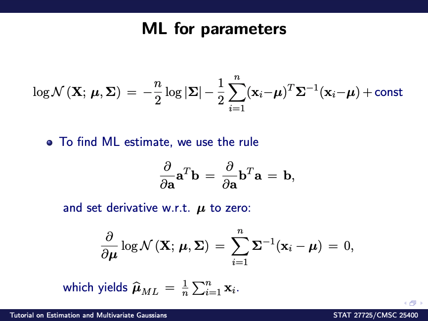
PCA recovery-projection process

Applying PCA to asset returns,

$\boldsymbol{\mathsf{Y}}=\boldsymbol{\mathsf{W}}\boldsymbol{\mathsf{R}}$

where $\boldsymbol{\mathsf{R}}\in \mathbb{R}^{S\times T}$ : a given data set with $S$ asset returns from $T$ trading days, $\boldsymbol{\mathsf{W}}\in \mathbb{R}^{S\times S}$ : a transfomation matrix of eigenvectors, and $\boldsymbol{\mathsf{Y}}\in \mathbb{R}^{S\times T}$ : the projected asset returns (or components in PCA)
- In matrix form, $\boldsymbol{\mathsf{Y}}=\boldsymbol{\mathsf{W}}\boldsymbol{\mathsf{R}}$ can be represented as below: $\begin{bmatrix} \vert & \vert & & \vert \\ c_1 & c_2 & \dots & c_T \\ \vert & \vert & & \vert \end{bmatrix} = \begin{bmatrix} \rule[.5ex]{3ex}{0.25pt} & e_1^\top & \rule[.5ex]{3ex}{0.25pt} \\ \rule[.5ex]{3ex}{0.25pt} & e_2^\top & \rule[.5ex]{3ex}{0.25pt} \\ & \vdots & \\ \rule[.5ex]{3ex}{0.25pt} & e_S^\top & \rule[.5ex]{3ex}{0.25pt} \end{bmatrix} \begin{bmatrix} \vert & \vert & & \vert \\ r_1 & r_2 & \dots & r_T \\ \vert & \vert & & \vert \end{bmatrix}$ where $c_i \in \mathbb{R}^S$ : component, $e_i \in \mathbb{R}^S$ : eignevector and $r_t \in \mathbb{R}^S$ : (observed) asset return at time $t$ .
In order to generate new artificial assets,

$\boldsymbol{\mathsf{W}}^{\prime}\boldsymbol{\mathsf{Y}}=\boldsymbol{\mathsf{R}}^{\prime}$

where $\boldsymbol{\mathsf{Y}}\in \mathbb{R}^{S\times T}$ : the projected asset returns (or components in PCA) (computed above), $\boldsymbol{\mathsf{W}}^{\prime}\in \mathbb{R}^{S^{\prime} \times S}$ : an artificial transformation matrix (generated below), and $\boldsymbol{\mathsf{R}}^{\prime}\in \mathbb{R}^{S^{\prime} \times T}$ : artificially generated assets
- In matrix form, can be represented as below: $\begin{bmatrix} \rule[.5ex]{3ex}{0.25pt} & \tilde{e}_1^\top & \rule[.5ex]{3ex}{0.25pt} \\ \rule[.5ex]{3ex}{0.25pt} & \tilde{e}_2^\top & \rule[.5ex]{3ex}{0.25pt} \\ & \vdots & \\ \rule[.5ex]{3ex}{0.25pt} & \tilde{e}_{S^{\prime}}^\top & \rule[.5ex]{3ex}{0.25pt} \end{bmatrix} \begin{bmatrix} \vert & \vert & & \vert \\ c_1 & c_2 & \dots & c_T \\ \vert & \vert & & \vert \end{bmatrix} = \begin{bmatrix} \vert & \vert & & \vert \\ \tilde{r}_1 & \tilde{r}_2 & \dots & \tilde{r}_T \\ \vert & \vert & & \vert \end{bmatrix}$ where $\tilde{e}_i \in \mathbb{R}^S$ : additional eigenvectors , $c_i \in \mathbb{R}^S$ : component, and $\tilde{r}_t \in \mathbb{R}^{S^{\prime}}$ : generated asset returns at time $t$ .
How to generate additional eigenvecotors?
$\tilde{e}\sim N (\mu_{\mathsf{W}}, \Sigma_{\mathsf{W}})$
where $\hat{\mu_{\mathsf{W}}}=\frac{1}{n}\sum_{s=1}^{S}e_s$ and $\hat{\Sigma_{\mathsf{W}}}=Cov(\boldsymbol{\mathsf{W}})$ .

Correction of expression

Paper	Python
For a given dataset $\boldsymbol{\mathsf{R}}$ of $S$ asset returns from $T$ trading days ( $S \times T$ ), a PCA transformation matrix $\boldsymbol{\mathsf{W}}$ can be obtained and these assets projected through $\boldsymbol{\mathsf{Y}}=\boldsymbol{\mathsf{W}}\boldsymbol{\mathsf{R}}$ , being $\boldsymbol{\mathsf{Y}}$ the projected asset returns or components. $\boldsymbol{\mathsf{Y}}=\boldsymbol{\mathsf{W}}\boldsymbol{\mathsf{R}}$ - $\boldsymbol{\mathsf{R}}$ : a given dataset with $S$ asset returns and $T$ trading days ( $S \times T$ ) - $\boldsymbol{\mathsf{W}}$ : a PCA transformation matrix ( $S \times S$ ) - $\boldsymbol{\mathsf{Y}}$ : the projected asset returns or components ( $S \times T$ ) If no dimension reduction is applied, $\boldsymbol{\mathsf{W}}$ is a transformation matrix of eigenvectors $\boldsymbol{\mathsf{w}}_{\mathsf{s}}$ that maps the original vectors of asset returns $\boldsymbol{\mathsf{r}}_{\mathsf{t}}$ into their components $\boldsymbol{\mathsf{y}}_{\mathsf{t}}$ . - $\boldsymbol{\mathsf{W}}=\boldsymbol{\mathsf{V}}\boldsymbol{\mathsf{V}}^{\top}$ , where $\boldsymbol{\mathsf{V}}$ is a matrix whose column is eigenvector $\boldsymbol{\mathsf{w}}_{\mathsf{s}}$ for $\mathsf{s}=1,...\mathsf{S}$	`R = df_wide.copy()` `pca = PCA(n_components = n_comp)` `pca_fit_transform = pca.fit_transform(R.T)` `Y = pca.inverse_transform(pca_fit_transform)`
The procedure used to generate those additional eigenvectors is to draw them from a multivariate normal distribution with parameters $\mu=\mathsf{E}[\boldsymbol{\mathsf{w}}_{\mathsf{s}}]$ and $\Sigma=\mathsf{Cov}(\boldsymbol{\mathsf{w}}_{\mathsf{i}},\boldsymbol{\mathsf{w}}_{\mathsf{j}})$ .	`COMPONENTS = pca.components_` `mu_hat_for_EV = list(map(lambda x : np.mean(x), COMPONENTS))` `Sigma_hat_for_EV = np.cov(COMPONENTS)` `W_prime = np.random.multivariate_normal(mu_hat_for_EV, Sigma_hat_for_EV, S_new)`
The components $Y$ are projected back to the original space by applying the inverse transformation. $W^{\prime}Y=R^{\prime}$ - $W^{\prime}$ : an artificial ~~transformation matrix~~ $\to$ eigenvectors - $Y$ : the components - $R^{\prime}$ : a new artificially generated set of assets	`generated = np.matmul(pca_inverse_transform, W_prime.T)`

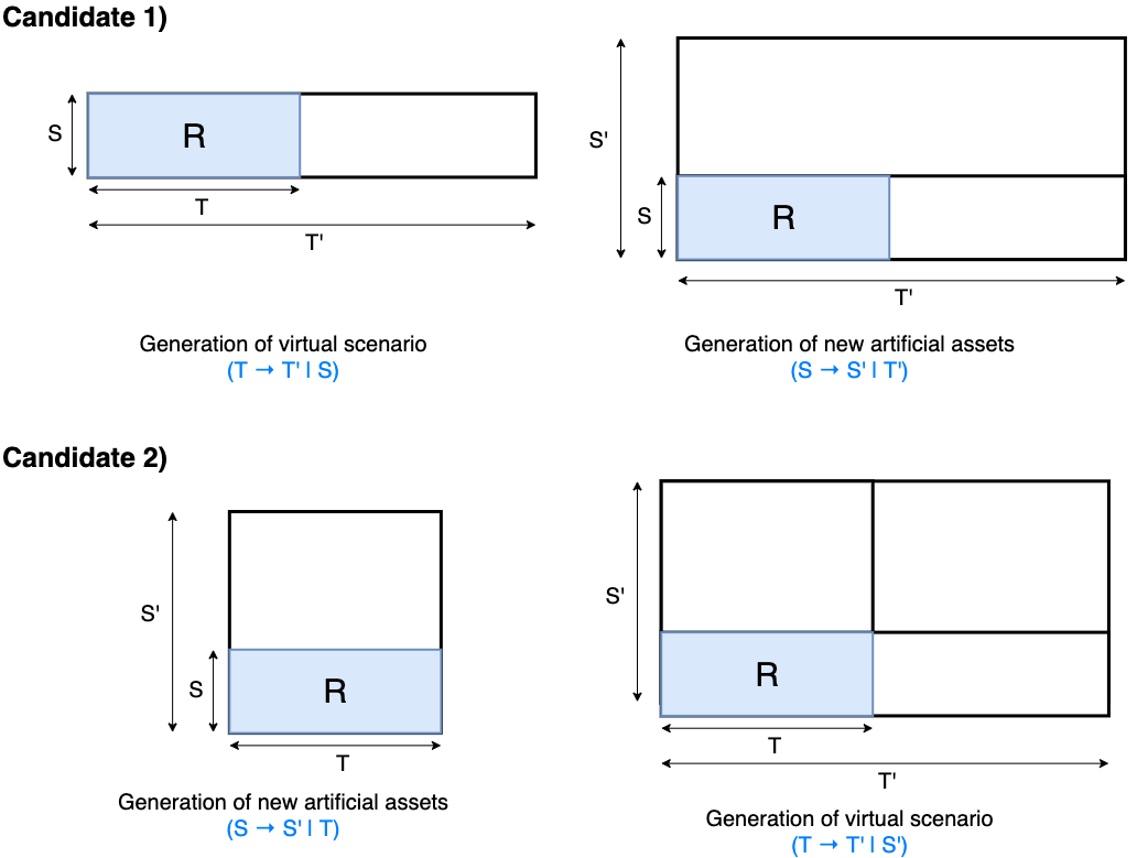
How to combine these techniques?

The final goal
Candidate scenarios
- Candidate2 seems more reasonable!

Python source code

from datetime import datetime
import os
import traceback    
    
N_rep = 3 # 1000 # number of repetitions
trial_id = 0
n_comp = 330 # number of PCs
S_new = 3 # 500 # size of artificial assets
N = 100 # 5000 # virtual scenario size (time length)

logger = make_logger()

for rep_idx in range(N_rep):
    random.seed(rep_idx + 1)
    logger.info("repeat = {} with random.seed({})".format(rep_idx + 1, rep_idx + 1))
    
    start_time = datetime.now()

    ### Generating artificial assets
    
    R = df_wide.copy()
    
    try:
        pca = PCA(n_components = n_comp)
        pca_fit_transform = pca.fit_transform(R.T)
        pca_inverse_transform = pca.inverse_transform(pca_fit_transform)

        COMPONENTS = pca.components_
        COMPONENTS.shape

        mu_hat_for_EV = list(map(lambda x : np.mean(x), COMPONENTS))
        Sigma_hat_for_EV = np.cov(COMPONENTS)
        
    except Exception as e:
        trace_back = traceback.format_exc()
        message = str(e)+ "\n" + str(trace_back)
        logger.error('[FAIL] %s', message)
    
    W_prime = np.random.multivariate_normal(mu_hat_for_EV, Sigma_hat_for_EV, S_new)
    generated = np.matmul(pca_inverse_transform, W_prime.T)
    
    R_prime = pd.DataFrame(generated.T.copy())
    P_prime_T = return_to_price(pd.DataFrame(generated))
    
    ### Estimation for multivariate normal
    
    mu_total = []
    Sigma_total = []
    window_sizes = []

    for seg in range(len(breakpoints) - 1): # [0]:

        R_prime_seg = R_prime.iloc[:, breakpoints[seg]:(breakpoints[seg+1] + 1)]

        seg_size = R_prime_seg.shape[1]
        W = seg_size - L
        window_sizes.append(W)
        # print('>>> Seg {} : {} data points, {} windows'.format(seg + 1, seg_size, W))

        mu_trend = []
        Sigma_trend = []

        for w in range(W):

            R_prime_window = R_prime_seg.iloc[:, w:(w+L)]
          
            mu_hat = R_prime_window.mean(axis=1)
            Sigma_hat = np.cov(R_prime_window)
          
            mu_trend.append(mu_hat)
            Sigma_trend.append(Sigma_hat)

        mu_total.append(mu_trend)
        Sigma_total.append(Sigma_trend)
    
    ### Random generation & Concatenation
    
    n_gen = int(np.ceil(N / sum(window_sizes)))
    n_seg = np.asarray(mu_total).shape[0]
    
    virtual_scenario = []

    for seg in range(n_seg):

        mu_trend = mu_total[seg]
        Sigma_trend = Sigma_total[seg]
        
        # print(">> Seg {}".format(seg + 1))

        window_size = np.asarray(mu_trend).shape[0]

        # print(">> window_size : {}".format(window_size))

        for w in range(window_size):
            mu_hat = mu_trend[w]
            Sigma_hat = Sigma_trend[w]

            generated_returns = np.random.multivariate_normal(mu_hat, Sigma_hat, n_gen)

            virtual_scenario.extend(generated_returns.tolist())
            
    vs_return0 = pd.DataFrame(virtual_scenario)
    selected_idx = np.random.permutation(vs_return0.shape[0])[:N]
    selected_idx.sort()
    vs_return = vs_return0.iloc[selected_idx, :].reset_index(drop=True)  # copy().take(selected_idx.sort()).reset_index(drop=True)
    vs_price = return_to_price(vs_return)
    virtual_market_index = vs_price.mean(axis=1)
    # print('a:{0:05d}'.format(a))
    
    save_dir = './results/repeats/rep_{0:04d}'.format(rep_idx + 1)
    if not os.path.exists(save_dir):
        os.makedirs(save_dir)
    
    vs_return.to_csv(save_dir + '/vs_return.csv'.format(rep_idx + 1))
    vs_price.to_csv(save_dir + '/vs_price.csv'.format(rep_idx + 1))
    virtual_market_index.to_csv(save_dir + '/vs_market_index.csv'.format(rep_idx + 1))
    
    end_time = datetime.now()
    time_diff = end_time - start_time
    tsecs = time_diff.total_seconds()

    print(">> Repetition {} (spent {} mins)".format(rep_idx + 1, round(tsecs / 60, 2)))
    
    del vs_return, vs_price, virtual_market_index