intro :
- 선형 회귀 훈련시키는 두 가지 방법
1) 직접 계산할 수 있는 공식으로 비용 함수 최소화하는(=훈련세트에 가장 잘 맞는) 모델 파라미터 구한다.
2) 경사 하강법 - 다항 회귀
-> 과대적합되기 쉬움. -> 규제 기법 - 로지스틱회귀, 소프트맥스 회귀
4.1 선형 회귀
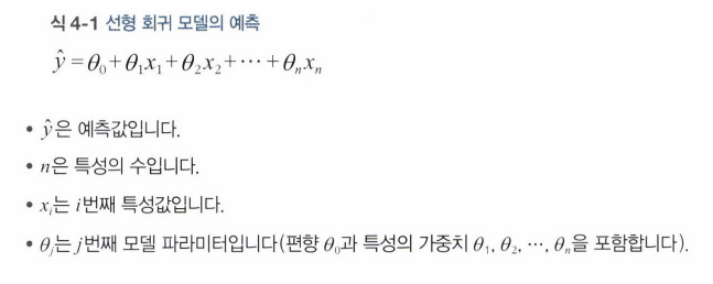
y = theta0 + theta1*x1
-> 훈련세트에 잘 맞는 파라미터 설정! RMSE를 최소화 하는 theta값 찾기 (cost 함수 최소화)
1) 해석적 방법 : 정규방정식 (특이행렬이라면 특이값분해(SVD) 통한 유사역행렬 사용)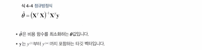
# 정규 방정식
import numpy as np
from matplotlib import pyplot as plt
X_b = np.c_[np.ones((100, 1)), X]  # 모든 샘플에 x0 = 1을 추가합니다.
theta_best = np.linalg.inv(X_b.T.dot(X_b)).dot(X_b.T).dot(y)
theta_best # array([[4.21509616],[2.77011339]])

X_new = np.array([[0], [2]])
X_new_b = np.c_[np.ones((2, 1)), X_new]  # 모든 샘플에 x0 = 1을 추가합니다.
y_predict = X_new_b.dot(theta_best)
y_predict # array([[4.21509616],[9.75532293]])
plt.plot(X_new, y_predict, "r-")
plt.plot(X, y, "b.")
plt.axis([0, 2, 0, 15])
plt.show()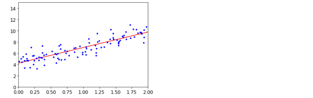
-> 두가지 방법 모두 특성 수 많아지면 매우 느려진다.
-> 특성이 매우 많고 훈련 샘플이 너무 많을 땐?
2) 경사 하강법
파라미터 벡터 theta에 대해 비용함수의 현재 기울기 계산. 기울기 감소하는 방향으로 진행. 0이 되면 최솟값 도달!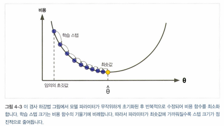
학습 스텝 : 기울기에 비례. 최솟값에 가까워질수록 스텝 크기 점진적 감소. 학습률(learning rate)하이퍼 파라미터로 결정됨
학습률 너무 작으면? 오래걸림/ 너무 크면? 골짜기를 지나침
-> 경사 하강법 문제점
1. 무작위 초기화로 global에 수렴하기 전 local에 수렴할 수 있다.
2. 평탄한 지점에서 일찍 멈출 위험
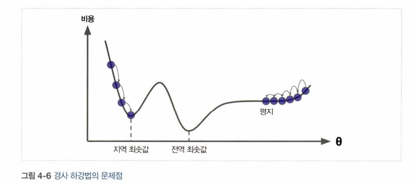
-> 다행히 선형회귀의 mse 함수는 볼록함수.. but 특성들의 스케일이 매우 다르면 길쭉할 수 있다. (시간이 오래걸림) 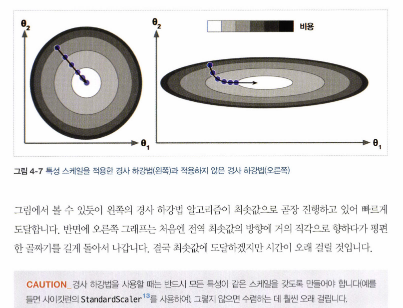
4.2.1 배치 경사 하강법
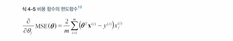
- 편도 함수 : 파라미터 값 변경 될 때 비용함수가 얼마나 바뀌는 지..
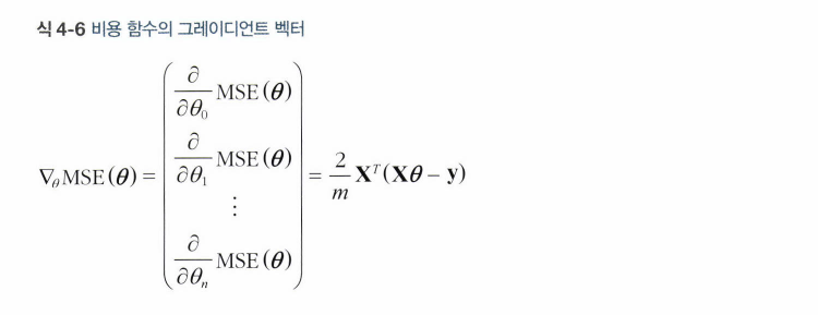
- 매 스텝에서 전체 훈련세트X에 대해 계산.
# 경사 하강법
eta = 0.1 # 학습률
n_iteration = 1000
m = 100
theta = np.random.randn(2,1) #무작위 초기화

for iteration in range(n_iteration):
    gradients = 2/m * x_b.T.dot(x_b.dot(theta)-y)
    theta = theta - eta * gradients
theta #array([[4.11862196],[3.02292557]]) 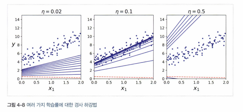
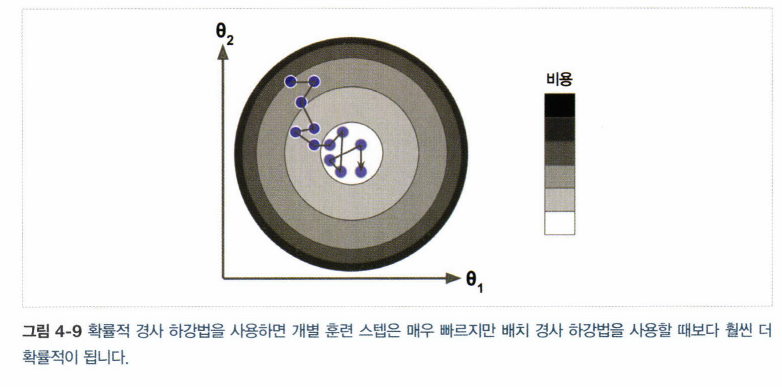
4.2.2 확률적 경사 하강법
# 확률적 경사 하강법
n_epochs = 50
t0,t1 = 5,50

def learning_schedule(t):
    return t0/(t+t1)

theta = np.random.randn(2,1)

for epoch in range(n_epochs):
    for i in range(m):
        rand_index = np.random.randint(m) # 0~99 중 랜덤 정수 한개
        xi = x_b[rand_index:rand_index+1]
        yi = y[rand_index:rand_index+1]
        gradients = 2 * xi.T.dot(xi.dot(theta)-yi)
        eta = learning_schedule(epoch*m+i) # 학습률 계속 변경
        theta = theta - eta*gradients

theta #array([[4.09999891],[3.03620409]])- 매 스텝에서 한 개의 샘플 무작위 선택, 하나의 샘플에 대한 기울기 계산. 속도 빠름 but 불안정
- 무작위성 -> 지역 최솟값 건너뛸 수 있어 전역 찾을 가능성 높아짐. but 전역에 다다르지 못할수도. -> 학습률 점진적 감소
4.2.3 미니배치 경사 하강법
- 미니배치라 부르는 임의의 작음 샘플 세트에 대해 기울기 계산.
#미니배치 경사 하강법
theta_path_mgd = []

n_iterations = 50
minibatch_size = 20

np.random.seed(42)
theta = np.random.randn(2,1)  # 랜덤 초기화

t0, t1 = 200, 1000
def learning_schedule(t):
    return t0 / (t + t1)

t = 0
for epoch in range(n_iterations):
    shuffled_indices = np.random.permutation(m)
    X_b_shuffled = X_b[shuffled_indices]
    y_shuffled = y[shuffled_indices]
    for i in range(0, m, minibatch_size):
        t += 1
        xi = X_b_shuffled[i:i+minibatch_size]
        yi = y_shuffled[i:i+minibatch_size]
        gradients = 2/minibatch_size * xi.T.dot(xi.dot(theta) - yi)
        eta = learning_schedule(t)
        theta = theta - eta * gradients
        theta_path_mgd.append(theta)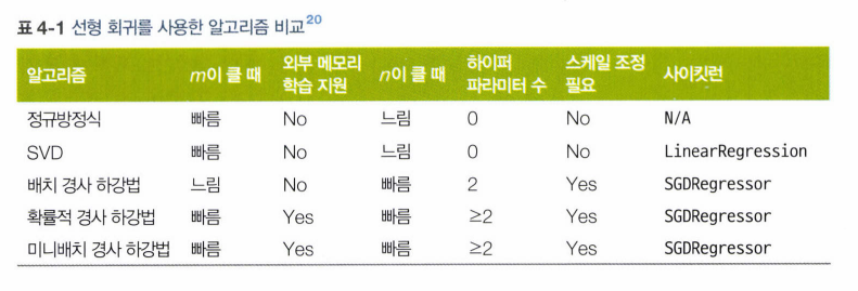
4.3 다항 회귀
데이터가 직선이 아닌 복잡한 형태 일 때
-> PolynomialFeatures 사용. 특성 간의 모든 교차항 추가하기 때문에 특성 사이의 관계도 파악 가능!
# 다항회귀
m = 100
x = 6* np.random.rand(m,1) - 3
y = 0.5 * x**2 + x+ 2 + np.random.randn(m,1)

from sklearn.preprocessing import PolynomialFeatures
poly_features = PolynomialFeatures(degree=2, include_bias =False)
x_poly = poly_features.fit_transform(x)

x_poly[0] # x특성에 제곱항 추가(교차항정보)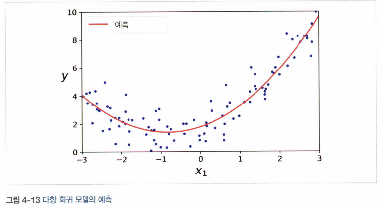
- 고차 다항 회귀 모델은 훈련데이터에 과대 적합.. 선형모델은 과소적합.. 2차가 적당.
과대적합/과소적합 판단 기준?
- 교차 검증
- 학습곡선 : 훈련, 검증 세트의 모델 성능을 훈련세트 크기의 함수로 나타냄
4.4 학습 곡선
- 과소적합 예
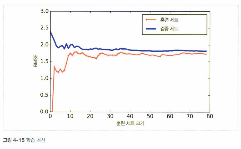
- 적은 수의 훈련 샘플로 훈련될 때에는 제대로 일반화될 수 없어서 검증 오차가 초기에 매우 크다.
- 모델에 훈련 샘플이 추가됨에 따라 학습이 되고 검증 오차가 천천히 감소한다. 하지만 선형 회귀의 직선은 데이터를 잘 모델링할 수 없으므로 오차의 감소가 완만해져서 훈련 세트의 그래프와 가까워진다.
- 과대적합 예
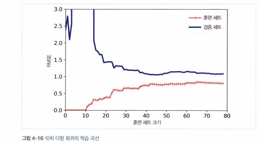 • 훈련 데이터의 오차가 선형 회귀 모델보다 훨씬 낮다. 훈련 데이터에서의 모델 성능이 검증 데이터에서보다 훨씬 좋다.
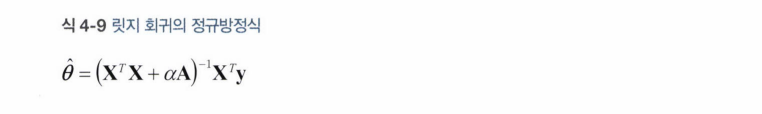
4.5 규제가 있는 선형 모델
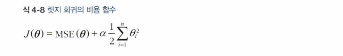
4.5.1 릿지
from sklearn.linear_model import Ridge
ridge_reg = Ridge(alpha=1, solver="cholesky", random_state=42)
ridge_reg.fit(X, y)
ridge_reg.predict([[1.5]])
ridge_reg = Ridge(alpha=1, solver="sag", random_state=42)
ridge_reg.fit(X, y)
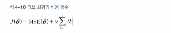
ridge_reg.predict([[1.5]])4.5.2 라쏘
from sklearn.linear_model import Lasso
lasso_reg = Lasso(alpha=0.1)
lasso_reg.fit(X, y)
lasso_reg.predict([[1.5]])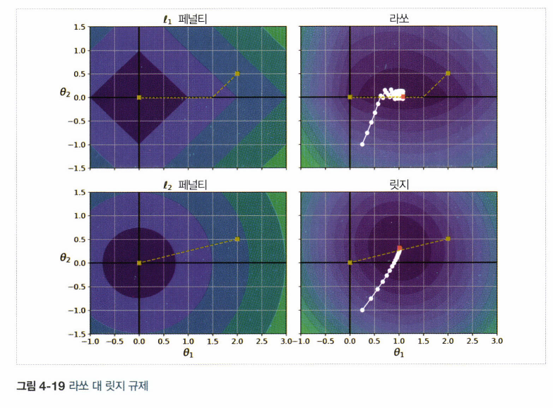
4.5.3 엘라스틱 넷
4.5.4 조기 종료
4.6 로지스틱 회귀
: 분류에 사용하는 회귀 알고리즘
