6.2 트리모델

트리모델

• 회귀 및 분석 트리, 의사 결정 트리, 트리 라고 불리는 대중적인 분류(및 회귀) 방법
• if-then-else 규칙의 집합체라고 할 수 있음 → 이해와 구현이 쉽다
  • 스무고개랑 비슷한 맥락
• 데이터에 존재하는 복잡한 상호 관계에 따른 숨겨진 패턴을 발견할 수 있다.
• 대출 데이터 분류를 위한 간단한 트리 모델
  • sklearn.tree.DecisionTreeClassifier

    predictors = ['borrower_score', 'payment_inc_ratio']
    outcome = 'outcome'
    
    X = loan3000[predictors]
    y = loan3000[outcome]
    
    loan_tree = DecisionTreeClassifier(random_state=1, criterion='entropy',
                                       min_impurity_decrease=0.003)
    loan_tree.fit(X, y)
    plotDecisionTree(loan_tree, feature_names=predictors, class_names=loan_tree.classes_)

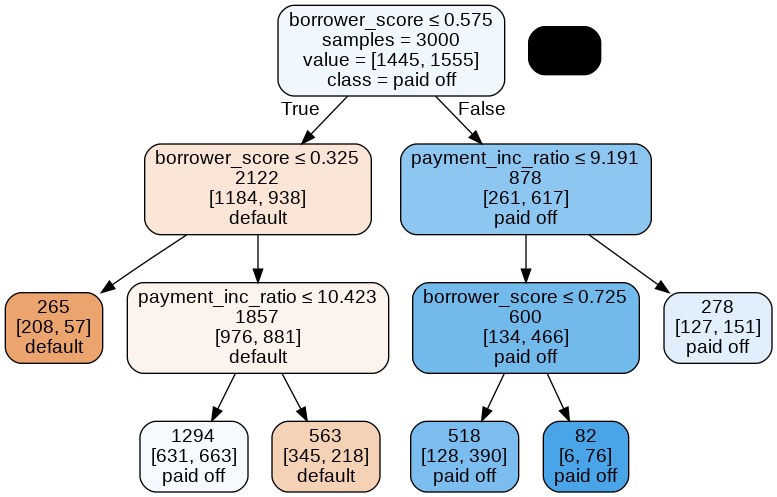
    노드가 참이면 왼쪽, 거짓이면 오른쪽으로 움직이면서 결정된다.
    
    →이걸 text로 나타내려면 `textDecisionTree()`를 사용
    
    ```jsx
    print(textDecisionTree(loan_tree))
    ```
    
    ```jsx
    node=0 test node: go to node 1 if 0 <= 0.5750000178813934 else to node 6
      node=1 test node: go to node 2 if 0 <= 0.32500000298023224 else to node 3
        node=2 leaf node: [[0.785, 0.215]]
        node=3 test node: go to node 4 if 1 <= 10.42264986038208 else to node 5
          node=4 leaf node: [[0.488, 0.512]]
          node=5 leaf node: [[0.613, 0.387]]
      node=6 test node: go to node 7 if 1 <= 9.19082498550415 else to node 10
        node=7 test node: go to node 8 if 0 <= 0.7249999940395355 else to node 9
          node=8 leaf node: [[0.247, 0.753]]
          node=9 leaf node: [[0.073, 0.927]]
        node=10 leaf node: [[0.457, 0.543]]
    ```
    

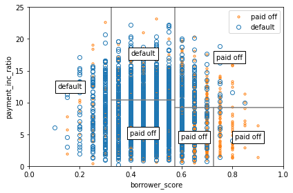
6.2.2 재귀 분할 알고리즘

💡 재귀 분할

마지막 분할 영역에 해당하는 출력이 최대한 비슷한 결과를 보이도록 데이터를 반복적으로 분할하는 것

• 예측변수 값을 기준으로 데이터를 반복적으로 분할한다.

분할 영역 A와 P개의 예측변수 집합 $X_j (j=1,...,P)$에 대해

1. 각 예측변수 $X_j$에 대해 $X_j$에 해당하는 어떤 변수(s)를 넣어 A를 $X_j$≥s, $X_j$<s인 두 집합으로 나눈다.

2. 분할 영역 안에서 동질성을 측정한다.

3. s를 바꿔가며 위 과정을 반복하고, 동질성이 가장 큰 $X_j$와 $s_j$를 선택한다.

4. $A_1$과 $A_2$에 대해 위 과정을 반복하며 계속해서 분할한다.

5. 충분한 분할(더이상 동질성이 개선되지 않음)을 진행했을 때, 알고리즘을 종료한다.

   fig, ax = plt.subplots(figsize=(6, 4))
   
   loan3000.loc[loan3000.outcome=='paid off'].plot(
       x='borrower_score', y='payment_inc_ratio', style='.', 
       markerfacecolor='none', markeredgecolor='C1', ax=ax)
   loan3000.loc[loan3000.outcome=='default'].plot(
       x='borrower_score', y='payment_inc_ratio', style='o', 
       markerfacecolor='none', markeredgecolor='C0', ax=ax)
   ax.legend(['paid off', 'default']);
   ax.set_xlim(0, 1)
   ax.set_ylim(0, 25)
   ax.set_xlabel('borrower_score')
   ax.set_ylabel('payment_inc_ratio')
   
   x0 = 0.575
   x1a = 0.325; y1b = 9.191
   y2a = 10.423; x2b = 0.725
   ax.plot((x0, x0), (0, 25), color='grey')
   ax.plot((x1a, x1a), (0, 25), color='grey')
   ax.plot((x0, 1), (y1b, y1b), color='grey')
   ax.plot((x1a, x0), (y2a, y2a), color='grey')
   ax.plot((x2b, x2b), (0, y1b), color='grey')
   
   labels = [('default', (x1a / 2, 25 / 2)),
             ('default', ((x0 + x1a) / 2, (25 + y2a) / 2)),
             ('paid off', ((x0 + x1a) / 2, y2a / 2)),
             ('paid off', ((1 + x0) / 2, (y1b + 25) / 2)),
             ('paid off', ((1 + x2b) / 2, (y1b + 0) / 2)),
             ('paid off', ((x0 + x2b) / 2, (y1b + 0) / 2)),
            ]
   for label, (x, y) in labels:
       ax.text(x, y, label, bbox={'facecolor':'white'},
               verticalalignment='center', horizontalalignment='center')
   
   plt.tight_layout()
   plt.show()

6.2.3 동질성과 불순도 측정하기

위에서 말한 ‘동질성(클래스 순도)’을 측정하는 방법이 필요함

동질성 최대화 = 불순도 최소화

지니불순도와 엔트로피가 대표적인 불순도 측정 지표

DecisionTreeClassifier은 gini를 기본값으로 분할 기준을 정함

지니불순도 (≠ 지니계수 : 이진 분류 문제에 한정됨)

$지니불순도 = 1 - (음성 클래스 비율^2 + 양성 클래스 비율^2 )$

EX) 100개의 샘플이 있는 어떤 노드의 두 클래스 비율이 0.5씩이라면 지니 불순도는 0.5가 됨 ⇒ 최악

$1-(0.5^2 + 0.5^2) = 0.5$

노드에 하나의 클래스만 있다면 지니 불순도는 0이 됨 ⇒ 완벽히 분류된 것

$1-(0^2+1^2)=0$

• 결정 트리 모델은 부모 노드와 자식 노드의 불순도 차이가 가능한 크도록 트리를 성장시킴 불순도 차이 계산 $부모 불순도 - (왼쪽 노드 샘플 수/부모샘플수) * 왼쪽노드불순도 - (오른쪽노드샘플수/부모샘플수) * 오른쪽노드불순도$ 부모 노드와 자식 노드의 불순도 차이를 정보 이득이라고 부름
  

엔트로피

$I(A) = p-log_2 (p)-(1-p)log_2 (1-p)$

두 값 모두 0에 가까울수록 좋음

각 분할로 만들어지는 영역에 대해 불순도를 측정하고 가중 평균을 계산한 후 단계마다 그 값이 가장 낮은 영역을 선택

def entropyFunction(x):
    if x == 0: return 0
    return -x * math.log(x, 2) - (1 - x) * math.log(1 - x, 2)

def giniFunction(x):
    return x * (1 - x)

x = np.linspace(0, 0.5, 50)
impure = pd.DataFrame({
    'x': x,
    'Accuracy': 2 * x,
    'Gini': [giniFunction(xi) / giniFunction(.5) for xi in x],
    'Entropy': [entropyFunction(xi) for xi in x],
})

fig, ax = plt.subplots(figsize=(4, 4))

impure.plot(x='x', y='Accuracy', ax=ax, linestyle='solid')
impure.plot(x='x', y='Entropy', ax=ax, linestyle='--')
impure.plot(x='x', y='Gini', ax=ax, linestyle=':')

plt.tight_layout()
plt.show()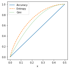

정확도가 높은 부분에서 지니 불순도와 엔트로피 측정값이 비슷하게 높아짐

6.2.4 트리 형성 중지하기

트리가 커질수록 점점 아주 작게 영역이 분할되는데 이는 세부 규칙이 만들어 지는 것

규칙이 세분화되면 학습 데이터에 대해 100% 정확도를 갖게 되는데 이는 학습 데이터의 노이즈까지 학습된 결과로 ‘과적합’된 것

새로운 데이터에 대해서도 좋은 성능을 갖기 위해서는 트리 성장을 멈춰야 함

파이썬에서 멈추는 방법

1. min_samples_split (기본값 2)과 min_samples_leaf (기본값 1)사용 최소 분할 영역 크기나 말단 잎 크기를 조절

   → 하위 영역 또는 말단 잎 크기가 너무 작다면 분할을 멈춤

2. min_impurity_decrease를 사용해 불순도 감소값에 따라 분할을 제한함

   → min_impurity_decrease값이 작을수록 트리는 복잡해짐

3. max_depth를 이용

but 예측 정확도를 최대화 하기 위한 최적값을 결정하기 매우 어렵기 때문에

(교차검증으로 파라미터 변경 + 가지치기로 트리 수정) 결합한 방법을 이용하는 것이 좋음

6.2.5 연속값 예측하기

트리 모델을 이용해 회귀분석을 하는 방법 또한 위에서 소개한 것과 동일한 과정을 거친다.

차이점

• 하위 분할 영역에서 평균으로부터의 편차들을 제곱한 값을 이용해서 불순도를 측정한다는 점
• RMSE( 제곱근평균제곱오차 ) 를 이용해 예측 성능을 평가한다는 점

트리 장점

• 어떤 변수가 중요한지, 변수 간에 어떤 관계가 있는지 시각화가 가능하다.
• 트리 모델은 일종의 규칙들의 집합이라고 볼 수 있기에 비전문가와 대화하는 데 효과적이다. → 그냥 모델링 한 것에 대한 결과를 보여주는 것보다 트리 모델을 보여주며 대화할 때 더 효과적
  

요약

• 의사 결정 트리는 결과를 분류하거나 예측하기 위한 일련의 규칙들을 생성한다.
• 이 규칙들은 데이터를 하위 영역으로 연속적으로 분할하는 것과 관련이 있다.
• 각 분할 혹은 분기는 어떤 한 예측변수 값을 기준으로 데이터를 두 부분으로 나누는 것이다.
• 각 단계마다, 트리 알고리즘은 결과의 불순도를 최소화하는 쪽으로 영역 분할을 진행한다.
• 더 이상 분할이 불가능할 때, 트리가 완전히 자랐다고 볼 수 있으며 각 말단 노드 혹은 잎 노드에 해당하는 레코드들은 단일 클래스에 속한다. ( ⇒ 완벽히 분류됐다. ) 새로운 데이터는 이 규칙 경로를 따라 해당 클래스로 할당된다.