Gradient 계산
s=f(x;W1,W2)=W2max(0,W1x)L=N1i=1∑NLi+λR(W1)+λR(W2)
- ∂W1∂L,∂W2∂L를 계산하면 W1,W2를 학습할 수 있다.
- 손실함수를 weight에 대해 미분한 도함수는 activation function이 바뀌면 다시 계산해야한다.
- 유지보수의 어려움
- Computational Graphs를 통해 모듈화하여 간단하게 계산할 수 있다.
Example
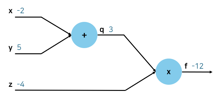
f(x,y,z)=(x+y)z,(x=−2,y=5,z=−4)
- Forward Pass: q=x+y,f=qz
- Backward Pass: Compute derivatives
- ∂x∂f,∂y∂f,∂z∂f를 구해야 한다.
- ∂f∂f=1
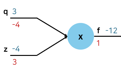
- ∂z∂f=q=3
- ∂q∂f=z=−4
- ∂y∂f=∂q∂f∂y∂q=∂q∂f=−4
- ∂x∂f=∂q∂f∂x∂q=∂q∂f=−4
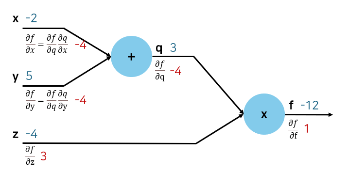
- Modularization
- Downstream Gradient: ∂x∂f (구하고자 하는 것, 해당 변수가 최종 결과에 얼마나 영향을 끼치는가)
- Local Gradient: ∂x∂q (당장 직접 계산할 수 있는 것)
- Upstream Gradient: ∂q∂f (이전 과정에서 계산된 것)
Activation Function의 Gradient
- Sigmoid: f′(x)=(1−σ(x))σ(x)
- ReLU: f′(x)={01for x<0for x≥0
Gradient Flow
- Add gate: Gradient distributor
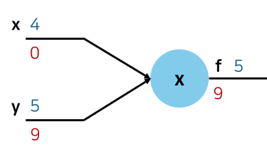
- Mul gate: swap multiplier
- Max gate: Gradient router
- Non linear 함수는 도함수를 정해둘 수 없어 매번 연산을 해야 한다.
- Modularization 조건: 미분(local gradient) 가능해야 한다.
Gradient code
s0 = w0 * x0
s1 = w1 * x1
s2 = s0 + s1
s3 = s2 + w2
L = sigmoid(s3)
- Downstream 계산을 위해 최종 output의 gradient는 1로 설정한다.
grad_L = 1.0
grad_s3 = grad_L * (1-L) * L
grad_w2 = grad_s3
grad_s2 = grad_s3
...
- Backward code
class Multiply(torch.autograd.Function):
@staticmethod
def backward(ctx, grad_z):
x, y = ctx.saved_tensors
grad_x = y * grad_z
grad_y = x * grad_x
return grad_x, grad_y
Vector Backpropagation
Vector Derivatives
- Regular derivative
- x∈R,y∈R
- x가 변화할 때 y가 변화하는 양 ∂x∂y∈R
- Gradient (Derivative)
- x∈RN,y∈R
- x가 변화할 때 y가 변화하는 양 ∂x∂y∈RN
- Jacobian (Derivative)
- x∈RN,y∈RM
- x가 변화할 때 y가 변화하는 양 ∂x∂y∈RN×M
J=⎣⎢⎢⎡∂x1∂F1⋮∂x1∂Fm⋯⋱⋯∂xn∂F1⋮∂xn∂Fm⎦⎥⎥⎤
- Example: F(x,y)=[x2y5x+sin(y)]
- Input 2차원, Output 2차원이므로 Jacobian은 [2×2]
- JF=[2xy5x2cos(y)]
Backprop with Vectors
- z=f(x,y)
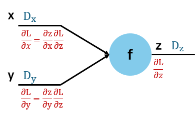
- 각 차원은 Dx,Dy,Dz이고 Loss L은 스칼라이다.
- Loss는 전체 손실을 계산하기 위해 scalar여야 한다.
- 손실이 N 차원이면 각 차원의 최적을 선택하는 것이 최적의 모델인 것이 아니다. 각 파라미터의 독립을 보장할 수 없다.
- Upstream Gradient: ∂z∂L,Dz 차원
- Local Gradients: ∂x∂z,Dx×Dz 차원, ∂y∂z,Dy×Dz 차원
- Downstream Gradients: [Dx×Dz]×[Dz×1]=Dx 차원, [Dy×Dz]×[Dz×1]=Dy 차원
- Downstream gradient의 차원은 그 값의 차원과 동일하다.
- Example: f(x)=max(0,x)
- Input: ⎣⎢⎢⎢⎡1−23−1⎦⎥⎥⎥⎤, Output: ⎣⎢⎢⎢⎡1030⎦⎥⎥⎥⎤
- Upstream gradient(주어지는 값): ⎣⎢⎢⎢⎡4−159⎦⎥⎥⎥⎤
- Local gradient: ⎣⎢⎢⎢⎡1000000000100000⎦⎥⎥⎥⎤
- Downstream gradient: ⎣⎢⎢⎢⎡4050⎦⎥⎥⎥⎤
Backpropagation with Matrices
- z=f(x,y)
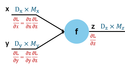
- 각 차원은 [Dx×Mx],[Dy×My],[Dz×Mz]이고 Loss L은 스칼라이다.
- Upstream gradient, Downstream gradient는 해당 차원과 동일하다.
- Local gradients
- ∂x∂z,[(Dx×Mx)×(Dz×Mz)]
- ∂y∂z,[(Dy×My)×(Dz×Mz)]