Monte Carlo Integration & Variance Reduction

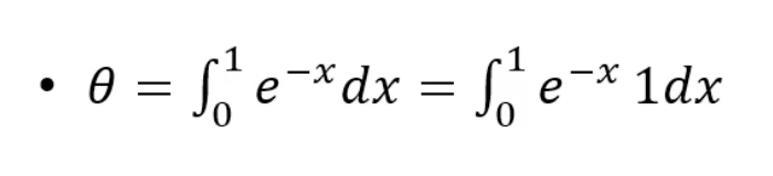
1. Simple Monte Carlo integration

m <- 10000
x <- runif(m)
theta.hat <- mean(exp(-x))

print(theta.hat)
print(-exp(-1) + 1)

2. Simple Monte Carlo integration, cont.

# or 뒤에 식으로 계산
m <- 10000
x <- runif(m, min=2, max=4)
theta.hat <- mean(exp(-x)) * 2

print(theta.hat)
print(- exp(-4) + exp(-2))

3. Monte Carlo integration, unbounded interval

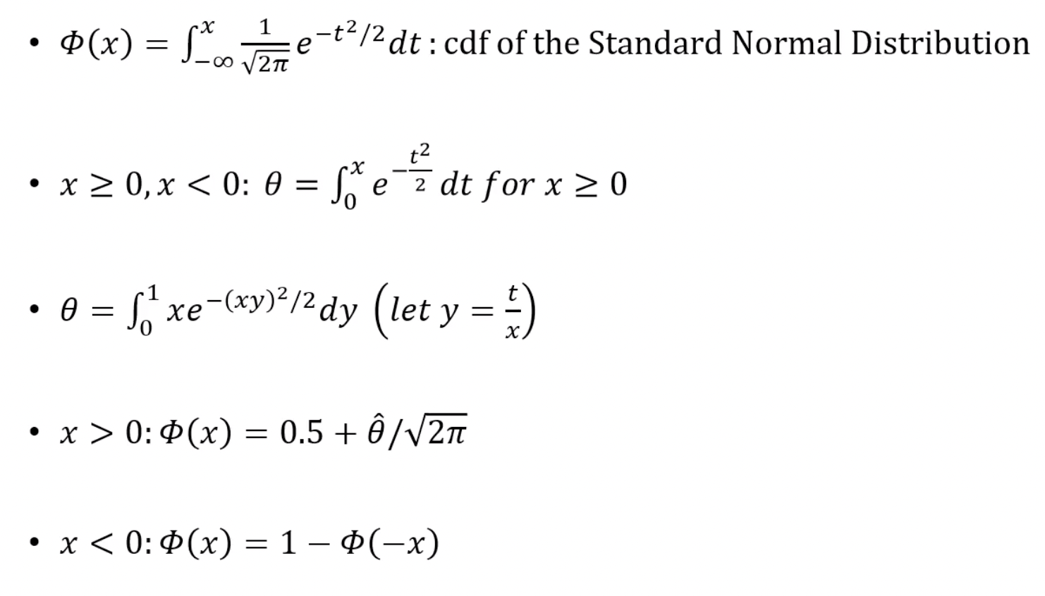
x <- seq(.1, 2.5, length = 10)

m <- 10000
u <- runif(m)
cdf <- numeric(length(x))

for (i in 1:length(x)) {
		g <- x[i] * exp(-(u * x[i])^2 / 2)
		cdf[i] <- mean(g) / sqrt(2 * pi) + 0.5
} 
Phi <- pnorm(x)

print(round(rbind(x, cdf, Phi), 3))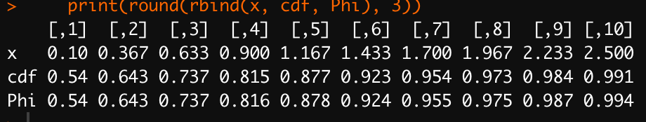

x <- seq(.1, 2.5, length = 10)

m <- 10000
z <- rnorm(m)
dim(x) <- length(x) # apply 쓰려고 차원 지정

p <- apply(x, MARGIN = 1, FUN = function(x, z) {mean(z < x)}, z = z)
Phi <- pnorm(x)

print(round(rbind(x, p, Phi), 3))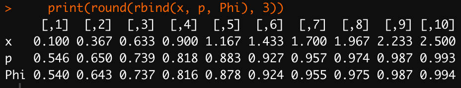

5. Error bounds for MC integration (MC error)

x <- 2
m <- 10000
z <- rnorm(m)
g <- (z < x)  #the indicator function, 여기서 g()
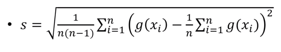
v <- mean((g - mean(g))^2) / m    # sqrt(v) = MC error
# 위에서 정확하게는 mean을 쓰면 안되지만 거의 차이 없다.
cdf <- mean(g) # 추정량

# Error bounds
c(cdf, v)
c(cdf - 1.96 * sqrt(v), cdf + 1.96 * sqrt(v)) # by CLT, cdf ~ Normal Dist

6. Antithetic variables

MC.Phi <- function(x, R = 10000, antithetic = TRUE) {
		u <- runif(R/2)
		if (!antithetic) v <- runif(R/2) else
				v <- 1 - u
		u <- c(u, v)
		cdf <- numeric(length(x))
		for (i in 1:length(x)) {
				g <- x[i] * exp(-(u * x[i])^2 / 2)
				cdf[i] <- mean(g) / sqrt(2 * pi) + 0.5
		}
cdf
}

x <- seq(.1, 2.5, length=5)
Phi <- pnorm(x)
set.seed(123)
MC1 <- MC.Phi(x, anti = FALSE)
set.seed(123)
MC2 <- MC.Phi(x)
print(round(rbind(x, MC1, MC2, Phi), 5))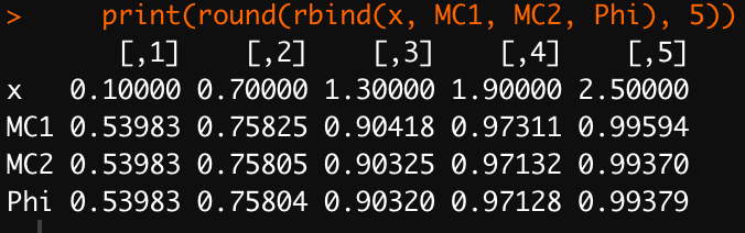

m <- 1000
MC1 <- MC2 <- numeric(m)
x <- 1.95
for (i in 1:m) {
		MC1[i] <- MC.Phi(x, R = 1000, anti = FALSE)
		MC2[i] <- MC.Phi(x, R = 1000)
}

print(sd(MC1)) # 0.0068
print(sd(MC2)) # 0.0004
print((var(MC1) - var(MC2))/var(MC1))

7. Control variate

m <- 10000
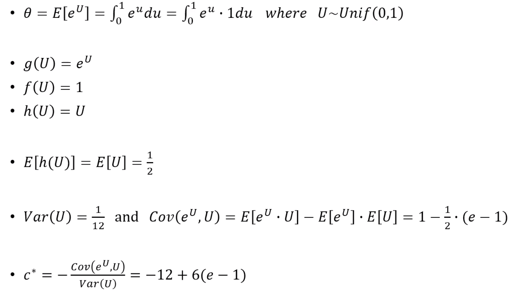
a <- - 12 + 6 * (exp(1) - 1)
U <- runif(m)
T1 <- exp(U)                  #simple MC
T2 <- exp(U) + a * (U - 1/2)  #controlled

mean(T1)
mean(T2)
(var(T1) - var(T2)) / var(T1) # 얼마나 줄었는지, 98% 줄었다.

8. MC integration using control variates

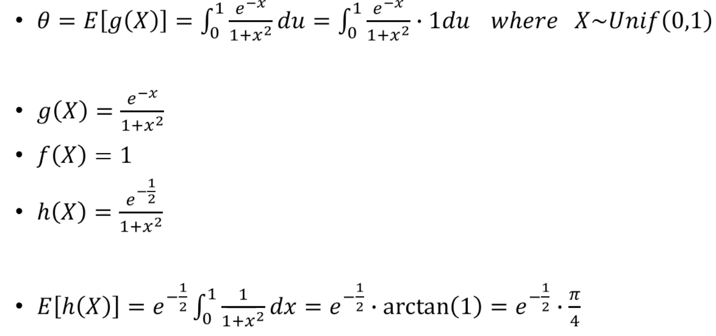
f <- function(u) exp(-.5)/(1+u^2)

g <- function(u) exp(-u)/(1+u^2)

set.seed(510) #needed later
u <- runif(10000)
B <- f(u)
A <- g(u)

cor(A, B)
a <- -cov(A,B) / var(B)    #est of c*
a

m <- 100000
u <- runif(m)
T1 <- g(u)
T2 <- T1 + a * (f(u) - exp(-.5)*pi/4)

c(mean(T1), mean(T2))
c(var(T1), var(T2))
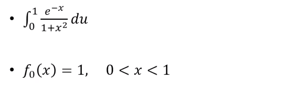
(var(T1) - var(T2)) / var(T1)

11. Choice of the importance function

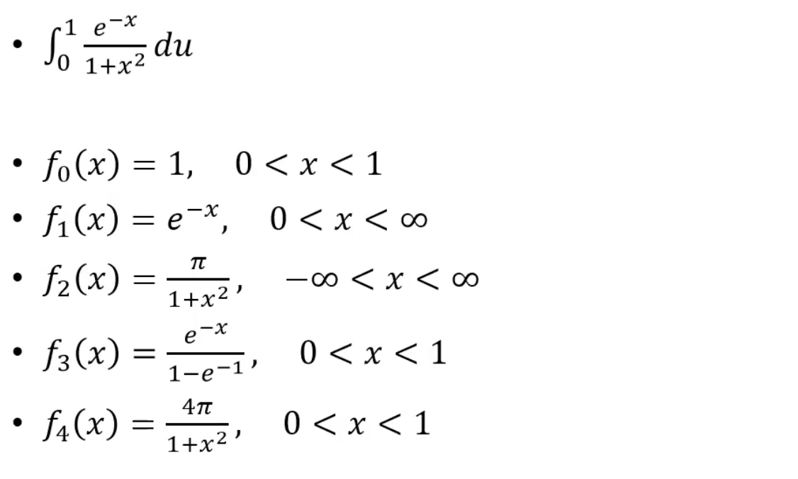
m <- 10000
theta.hat <- se <- numeric(5)
g <- function(x) {
		exp(-x - log(1+x^2)) * (x > 0) * (x < 1)
}

x <- runif(m)     #using f0
fg <- g(x)
theta.hat[1] <- mean(fg)
se[1] <- sd(fg)

x <- rexp(m, 1)   #using f1
fg <- g(x) / exp(-x)
theta.hat[2] <- mean(fg)
se[2] <- sd(fg)

x <- rcauchy(m)   #using f2
i <- c(which(x > 1), which(x < 0))
x[i] <- 2  #to catch overflow errors in g(x)
fg <- g(x) / dcauchy(x)
theta.hat[3] <- mean(fg)
se[3] <- sd(fg)

u <- runif(m)     #f3, inverse transform method
x <- - log(1 - u * (1 - exp(-1)))
fg <- g(x) / (exp(-x) / (1 - exp(-1)))
theta.hat[4] <- mean(fg)
se[4] <- sd(fg)

u <- runif(m)    #f4, inverse transform method
x <- tan(pi * u / 4)
fg <- g(x) / (4 / ((1 + x^2) * pi))
theta.hat[5] <- mean(fg)
se[5] <- sd(fg)

rbind(theta.hat, se / sqrt(m))

12. Stratified Sampling

M <- 20   #number of replicates
T2 <- numeric(4)
estimates <- matrix(0, 10, 2)

g <- function(x) {
		exp(-x - log(1+x^2)) * (x > 0) * (x < 1) }

for (i in 1:10) {
		estimates[i, 1] <- mean(g(runif(M)))
		T2[1] <- mean(g(runif(M/4, 0, .25)))
		T2[2] <- mean(g(runif(M/4, .25, .5)))
		T2[3] <- mean(g(runif(M/4, .5, .75)))
		T2[4] <- mean(g(runif(M/4, .75, 1)))
		estimates[i, 2] <- mean(T2)
}

estimates
apply(estimates, 2, mean)
apply(estimates, 2, var)

M <- 10000  #number of replicates
k <- 10     #number of strata
r <- M / k  #replicates per stratum
N <- 50     #number of times to repeat the estimation
T2 <- numeric(k)
estimates <- matrix(0, N, 2)

g <- function(x) {
		exp(-x - log(1+x^2)) * (x > 0) * (x < 1)
}

for (i in 1:N) {
		estimates[i, 1] <- mean(g(runif(M)))
		for (j in 1:k)
		    T2[j] <- mean(g(runif(M/k, (j-1)/k, j/k)))
    estimates[i, 2] <- mean(T2)
}

apply(estimates, 2, mean)
apply(estimates, 2, var)